What Matters In On-Policy Reinforcement Learning? A Large-Scale Empirical Study
在线策略强化学习中什么最重要?一项大规模实证研究
Marcin An dry ch owicz, Anton Raichuk, Piotr Stanczyk, Manu Orsini, Sertan Girgin, Raphael Marinier, Léonard Hussenot, Matthieu Geist, Olivier Pietquin, Marcin Michalski, Sylvain Gelly, Olivier Bachem
Marcin Andrychowicz, Anton Raichuk, Piotr Stanczyk, Manu Orsini, Sertan Girgin, Raphael Marinier, Léonard Hussenot, Matthieu Geist, Olivier Pietquin, Marcin Michalski, Sylvain Gelly, Olivier Bachem
Google Research, Brain Team
Google Research, Brain Team
Abstract
摘要
In recent years, on-policy reinforcement learning (RL) has been successfully applied to many different continuous control tasks. While RL algorithms are often conceptually simple, their state-of-the-art implementations take numerous low- and high-level design decisions that strongly affect the performance of the resulting agents. Those choices are usually not extensively discussed in the literature, leading to discrepancy between published descriptions of algorithms and their implementations. This makes it hard to attribute progress in RL and slows down overall progress [27]. As a step towards filling that gap, we implement ${>}50$ such “choices” in a unified on-policy RL framework, allowing us to investigate their impact in a large-scale empirical study. We train over $250^{\ '}000$ agents in five continuous control environments of different complexity and provide insights and practical recommendations for on-policy training of RL agents.
近年来,策略强化学习 (on-policy reinforcement learning, RL) 已成功应用于多种连续控制任务。尽管RL算法在概念上通常很简单,但其最先进的实现涉及大量底层和顶层设计决策,这些决策会显著影响最终智能体的性能。这些选择在文献中通常未被充分讨论,导致算法描述与其实现之间存在差异[27]。这使RL领域的进展难以归因,并拖慢了整体发展速度。为填补这一空白,我们在统一的策略RL框架中实现了${>}50$项此类"选择",通过大规模实验研究其影响。我们在五个不同复杂度的连续控制环境中训练了超过$250^{\ '}000$个智能体,为策略RL训练提供了洞见和实践建议。
1 Introduction
1 引言
Deep reinforcement learning (RL) has seen increased interest in recent years due to its ability to have neural-network-based agents learn to act in environments through interactions. For continuous control tasks, on-policy algorithms such as REINFORCE [2], TRPO [10], A3C [14], PPO [17] and off-policy algorithms such as DDPG [13] and SAC [21] have enabled successful applications such as quadrupedal locomotion [20], self-driving [30] or dexterous in-hand manipulation [20, 25, 32].
深度强化学习 (RL) 近年来受到越来越多的关注,因为它能让基于神经网络的AI智能体通过与环境交互学习行动策略。在连续控制任务中,REINFORCE [2]、TRPO [10]、A3C [14]、PPO [17] 等在线策略算法,以及 DDPG [13] 和 SAC [21] 等离线策略算法,已成功应用于四足机器人运动 [20]、自动驾驶 [30] 和灵巧手部操控 [20, 25, 32] 等领域。
Many of these papers investigate in depth different loss functions and learning paradigms. Yet, it is less visible that behind successful experiments in deep RL there are complicated code bases that contain a large number of low- and high-level design decisions that are usually not discussed in research papers. While one may assume that such “choices” do not matter, there is some evidence that they are in fact crucial for or even driving good performance [27].
许多论文深入研究了不同的损失函数和学习范式。然而,人们较少注意到的是,深度强化学习成功实验背后往往隐藏着复杂的代码库,其中包含大量通常不会在研究论文中讨论的低层次和高层次设计决策。虽然有人可能认为这些"选择"无关紧要,但有证据表明它们实际上对良好性能至关重要,甚至可能是关键驱动因素 [27]。
While there are open-source implementations available that can be used by practitioners, this is still unsatisfactory: In research publications, often different algorithms implemented in different code bases are compared one-to-one. This makes it impossible to assess whether improvements are due to the algorithms or due to their implementations. Furthermore, without an understanding of lower-level choices, it is hard to assess the performance of high-level algorithmic choices as performance may strongly depend on the tuning of hyper parameters and implementation-level details. Overall, this makes it hard to attribute progress in RL and slows down further research [15, 22, 27].
虽然从业者可以使用开源实现,但这仍不尽如人意:在研究出版物中,经常将不同代码库实现的算法进行一对一比较。这使得无法判断改进是源于算法本身还是其实现方式。此外,若不了解底层选择,则难以评估高层算法选择的性能,因为性能可能高度依赖于超参数调整和实现层面的细节。总体而言,这导致难以归因强化学习(RL)的进展,并延缓了进一步研究[15, 22, 27]。
Our contributions. Our key goal in this paper is to investigate such lower level choices in depth and to understand their impact on final agent performance. Hence, as our key contributions, we (1) implement ${>}50$ choices in a unified on-policy algorithm implementation, (2) conducted a large-scale (more than $250^{\ '}000$ agents trained) experimental study that covers different aspects of the training process, and (3) analyze the experimental results to provide practical insights and recommendations for the on-policy training of RL agents.
我们的贡献。本文的核心目标是深入研究这些底层选择,并理解它们对最终智能体性能的影响。因此,我们的主要贡献包括:(1) 在统一的同策略算法实现中实现了${>}50$种选择,(2) 进行了一项大规模实验研究(训练了超过$250^{\ '}000$个智能体),涵盖了训练过程的不同方面,(3) 分析实验结果,为强化学习智能体的同策略训练提供实用的见解和建议。
Most surprising finding. While many of our experimental findings confirm common RL practices, some of them are quite surprising, e.g. the policy initialization scheme significantly influences the performance while it is rarely even mentioned in RL publications. In particular, we have found that initializing the network so that the initial action distribution has zero mean, a rather low standard deviation and is independent of the observation significantly improves the training speed (Sec. 3.2).
最令人惊讶的发现。虽然我们的许多实验结果验证了常见的强化学习实践,但其中一些发现相当出人意料,例如策略初始化方案会显著影响性能,而这在强化学习文献中却鲜少被提及。具体而言,我们发现将网络初始化为使初始动作分布具有零均值、较低标准差且与观测无关的状态,能显著提升训练速度 (详见第3.2节)。
The rest of of this paper is structured as follows: We describe our experimental setup and performance metrics used in Sec. 2. Then, in Sec. 3 we present and analyse the experimental results and finish with related work in Sec. 4 and conclusions in Sec. 5. The appendices contain the detailed description of all design choices we experiment with (App. B), default hyper parameters (App. C) and the raw experimental results (App. D - K).
本文的其余部分结构如下:第2节描述实验设置和使用的性能指标。接着,第3节展示并分析实验结果,第4节介绍相关工作,第5节总结结论。附录包含所有实验设计选择的详细说明(附录B)、默认超参数(附录C)以及原始实验结果(附录D-K)。
2 Study design
2 研究设计
Considered setting. In this paper, we consider the setting of on-policy reinforcement learning for continuous control. We define on-policy learning in the following loose sense: We consider policy iteration algorithms that iterate between generating experience using the current policy and using the experience to improve the policy. This is the standard modus operandi of algorithms usually considered on-policy such as PPO [17]. However, we note that algorithms often perform several model updates and thus may operate technically on off-policy data within a single policy improvement iteration. As benchmark environments, we consider five widely used continuous control environments from OpenAI Gym [12] of varying complexity: Hopper-v1, Walker2d-v1, Half Cheetah-v1, Ant-v1, and Humanoid-v1 1.
考虑场景。本文研究了连续控制中的同策略强化学习场景。我们以下列宽松方式定义同策略学习:考察在生成当前策略经验与利用经验改进策略之间迭代的策略优化算法。这是PPO[17]等典型同策略算法的标准操作模式。但需注意,算法通常执行多次模型更新,因此在单个策略改进迭代中技术上可能处理异策略数据。作为基准环境,我们选用OpenAI Gym[12]中五个复杂度各异的经典连续控制环境:Hopper-v1、Walker2d-v1、Half Cheetah-v1、Ant-v1以及Humanoid-v1。
Unified on-policy learning algorithm. We took the following approach to create a highly configurable unified on-policy learning algorithm with as many choices as possible:
统一在线策略学习算法。我们采用以下方法创建了一个高度可配置的统一在线策略学习算法,尽可能提供多种选择:
The resulting agent implementation is detailed in Appendix B. The key property is that the implementation exposes all choices as configuration options in an unified manner. For convenience, we mark each of the choice in this paper with a number (e.g., C1) and a fixed name (e.g. num_envs (C1)) that can be easily used to find a description of the choice in Appendix B.
最终实现的AI智能体细节详见附录B。其核心特性在于以统一方式将所有选项暴露为可配置项。为便于查阅,我们在本文中用数字(如C1)和固定名称(如num_envs (C1))标注每个选项,这些标记可快速定位到附录B中对应的选项说明。
Difficulty of investigating choices. The primary goal of this paper is to understand how the different choices affect the final performance of an agent and to derive recommendations for these choices. There are two key reasons why this is challenging:
探究选择方案的难点。本文的主要目标是理解不同选择如何影响智能体的最终性能,并为这些选择提供建议。这具有挑战性的两个关键原因是:
First, we are mainly interested in insights on choices for good hyper parameter configurations. Yet, if all choices are sampled randomly, the performance is very bad and little (if any) training progress is made. This may be explained by the presence of sub-optimal settings (e.g., hyper parameters of the wrong scale) that prohibit learning at all. If there are many choices, the probability of such failure increases exponentially.
首先,我们主要关注的是如何选择良好的超参数配置。然而,如果所有选择都是随机采样的,性能会非常差,训练进展甚微(如果有的话)。这可能是因为存在次优设置(例如,超参数尺度错误)完全阻碍了学习。如果选择很多,这种失败的概率会呈指数级增长。
Second, many choices may have strong interactions with other related choices, for example the learning rate and the minibatch size. This means that such choices need to be tuned together and experiments where only a single choice is varied but interacting choices are kept fixed may be misleading.
其次,许多选择可能与其他相关选择存在强烈交互作用,例如学习率 (learning rate) 和小批量大小 (minibatch size)。这意味着此类选择需要共同调优,若实验中仅改变单个选择而保持交互选择固定,可能会产生误导性结果。
Basic experimental design. To address these issues, we design a series of experiments as follows: We create groups of choices around thematic groups where we suspect interactions between different choices, for example we group together all choices related to neural network architecture. We also include Adam learning rate (C24) in all of the groups as we suspect that it may interact with many other choices.
基础实验设计。为解决这些问题,我们设计了如下系列实验:围绕主题组创建选择群组(例如将神经网络架构相关选择归为一组),这些组别可能存在不同选择间的交互作用。我们在所有组别中都加入了Adam学习率(C24)参数,因其可能与其他多项选择产生交互。
Then, in each experiment, we train a large number of models where we randomly sample the choices within the corresponding group 2. All other settings (for choices not in the group) are set to settings of a competitive base configuration (detailed in Appendix C) that is close to the default PPOv2 configuration 3 scaled up to 256 parallel environments. This has two effects: First, it ensures that our set of trained models contains good models (as verified by performance statistics in the corresponding results). Second, it guarantees that we have models that have different combinations of potentially interacting choices.
然后,在每次实验中,我们训练大量模型,随机采样对应组2内的选项。其余未包含在该组的选项均采用接近默认PPOv2配置3的竞争性基准配置(详见附录C),并扩展至256个并行环境。这样做有两个效果:首先,它确保我们训练的模型集中包含优质模型(通过相应结果的性能统计验证);其次,它保证我们拥有具备潜在交互选项不同组合的模型。
We then consider two different analyses for each choice (e.g, for advantage estimator (C6)):
我们随后针对每个选择进行两种不同的分析(例如,对于优势估计器 (C6)):
Conditional 95th percentile: For each potential value of that choice (e.g., advantage estimator $({\mathsf{C}}6)=\mathbb{N}{\mathsf{-S t e p}},$ ), we look at the performance distribution of sampled configurations with that value. We report the 95th percentile of the performance as well as a confidence interval based on a binomial approximation 4. Intuitively, this corresponds to a robust estimate of the performance one can expect if all other choices in the group were tuned with random search and a limited budget of roughly 20 hyper parameter configurations.
条件95百分位:针对该选项的每个可能取值(例如优势估计器$({\mathsf{C}}6)=\mathbb{N}{\mathsf{-S t e p}},$),我们观察具有该取值的采样配置的性能分布。报告性能的95百分位值以及基于二项式近似的置信区间[4]。直观而言,这相当于当组内其他选项通过随机搜索和约20组超参数配置的有限预算进行调优时,可预期的稳健性能估计。
Distribution of choice within top $5%$ configurations. We further consider for each choice the distribution of values among the top $5%$ configurations trained in that experiment. The reasoning is as follows: By design of the experiment, values for each choice are distributed uniformly at random. Thus, if certain values are over-represented in the top models, this indicates that the specific choice is important in guaranteeing good performance.
前5%配置中的选择分布。我们进一步考虑每个选择在该实验训练的前5%配置中的数值分布。理由如下:根据实验设计,每个选择的数值是均匀随机分布的。因此,如果某些数值在顶级模型中占比过高,则表明该特定选择对保证良好性能至关重要。
Performance measures. We employ the following way to compute performance: For each hyperparameter configuration, we train 3 models with independent random seeds where each model is trained for one million (Hopper, Half Cheetah, Walker2d) or two million environment steps (Ant, Humanoid). We evaluate trained policies every hundred thousand steps by freezing the policy and computing the average un discounted episode return of 100 episodes (with the stochastic policy). We then average these score to obtain a single performance score of the seed which is proportional to the area under the learning curve. This ensures we assign higher scores to agents that learn quickly. The performance score of a hyper parameter configuration is finally set to the median performance score across the 3 seeds. This reduces the impact of training noise, i.e., that certain seeds of the same configuration may train much better than others.
性能指标。我们采用以下方法计算性能:对于每种超参数配置,使用独立随机种子训练3个模型,其中每个模型训练一百万步(Hopper、Half Cheetah、Walker2d)或两百万步环境交互(Ant、Humanoid)。每十万步通过冻结策略并计算100个回合的平均无折扣回报(使用随机策略)来评估训练策略。随后将这些分数平均,得到与学习曲线下面积成正比的单一种子性能分数,这确保了对快速学习的智能体赋予更高分数。最终将超参数配置的性能分数设定为3个种子性能分数的中位数,以此降低训练噪声的影响(即相同配置下某些种子的训练效果可能远优于其他种子)。
3 Experiments
3 实验
We run experiments for eight thematic groups: Policy Losses (Sec. 3.1), Networks architecture (Sec. 3.2), Normalization and clipping (Sec. 3.3), Advantage Estimation (Sec. 3.4), Training setup (Sec. 3.5), Timesteps handling (Sec. 3.6), Optimizers (Sec. 3.7), and Regular iz ation (Sec. 3.8). For each group, we provide a full experimental design and full experimental plots in Appendices D - K so that the reader can draw their own conclusions from the experimental results. In the following sections, we provide short descriptions of the experiments, our interpretation of the results, as well as practical recommendations for on-policy training for continuous control.
我们针对八个主题组进行了实验:策略损失(第3.1节)、网络架构(第3.2节)、归一化与截断(第3.3节)、优势估计(第3.4节)、训练设置(第3.5节)、时间步处理(第3.6节)、优化器(第3.7节)以及正则化(第3.8节)。对于每个组,我们在附录D-K中提供了完整的实验设计和实验图表,以便读者能够从实验结果中得出自己的结论。在接下来的章节中,我们将简要描述实验内容、对结果的解读,并为连续控制的在线策略训练提供实用建议。
3.1 Policy losses (based on the results in Appendix D)
3.1 策略损失 (基于附录D中的结果)
Study description. We investigate different policy losses (C14): vanilla policy gradient (PG), V-trace [19], PPO [17], AWR [33], V-MPO5 [34] and the limiting case of AWR $\beta\to0)$ ) and V-MPO $\left(\epsilon_{n}\rightarrow0\right)$ ) which we call Repeat Positive Advantages (RPA) as it is equivalent to the negative logprobability of actions with positive advantages. See App. B.3 for a detailed description of the different losses. We further sweep the hyper parameters of each of the losses (C15, C16, C18, C17, C19), the learning rate (C24) and the number of passes over the data (C3).
研究描述。我们研究了不同的策略损失 (C14):普通策略梯度 (PG)、V-trace [19]、PPO [17]、AWR [33]、V-MPO5 [34] 以及 AWR ($\beta\to0$) 和 V-MPO ($\left(\epsilon_{n}\rightarrow0\right)$) 的极限情况,后者我们称为重复正优势 (RPA),因为它等同于具有正优势动作的负对数概率。不同损失的详细描述参见附录 B.3。我们还进一步扫描了每种损失的超参数 (C15, C16, C18, C17, C19)、学习率 (C24) 以及数据遍历次数 (C3)。
The goal of this study is to better understand the importance of the policy loss function in the on-policy setting considered in this paper. The goal is not to provide a general statement that one of the losses is better than the others as some of them were specifically designed for other settings (e.g., the V-trace loss is targeted at near-on-policy data in a distributed setting).
本研究旨在更好地理解本文所探讨的同策略(on-policy)设置中策略损失函数的重要性。目标并非笼统判定某种损失函数优于其他类型,因为部分损失函数是专为其他场景设计(例如V-trace损失函数针对分布式环境中的近同策略数据)。
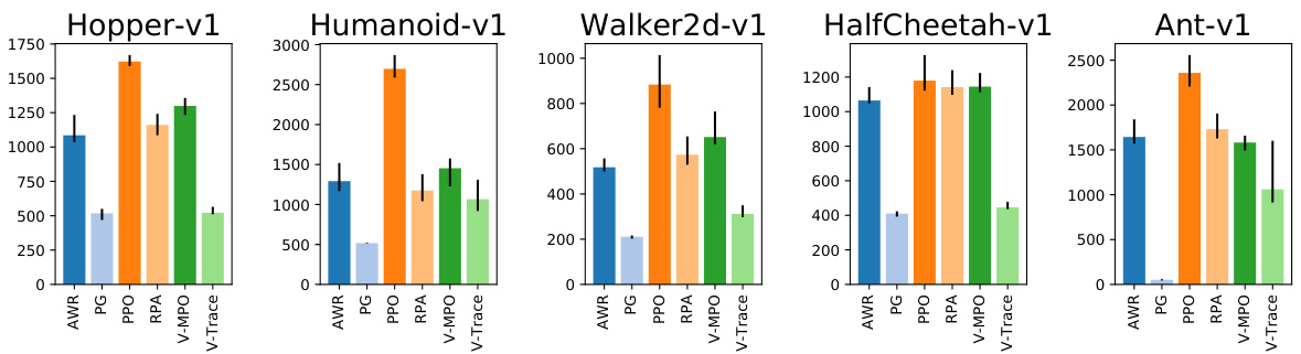
Figure 1: Comparison of different policy losses (C14).
图 1: 不同策略损失对比 (C14)。
Interpretation. Fig. 1 shows the 95-th percentile of the average policy score during training for different policy losses (C14). We observe that PPO performs better than the other losses on 4 out of 5 environments and is one of the top performing losses on Half Cheetah. As we randomly sample the loss specific hyper parameters in this analysis, one might argue that our approach favours choices that are not too sensitive to hyper parameters. At the same time, there might be losses that are sensitive to their hyper parameters but for which good settings may be easily found. Fig. 5 shows that even if we condition on choosing the optimal loss hyper parameters for each $\mathrm{loss}^{6}$ , PPO still outperforms the other losses on the two hardest tasks — Humanoid and $\mathrm{Ant^{7}}$ and is one of the top performing losses on the other 3 tasks. Moreover, we show the empirical cumulative density functions of agent performance conditioned on the policy loss used in Fig. 4. Perhaps un surprisingly, PG and ${\mathrm{V}}.$ -trace perform worse on all tasks. This is likely caused by their inability to handle data that become off-policy in one iteration, either due to multiple passes (C3) over experience (which can be seen in Fig. 14) or a large experience buffer (C2) in relation to the batch size (C4). Overall, these results show that trust-region optimization (preventing the current policy from diverging too much from the behavioral one) which is present in all the other policy losses is crucial for good sample complexity. For PPO and its clipping threshold $\epsilon$ (C16), we further observe that $\epsilon=0.2$ and $\epsilon=0.3$ perform reasonably well in all environments but that lower $\epsilon=0.1$ ) or higher $\epsilon=0.5$ ) values give better performance on some of the environments (See Fig. 10 and Fig. 32).
解读。图 1 展示了不同策略损失 (C14) 在训练期间平均策略得分的第 95 百分位数。我们观察到 PPO 在 5 个环境中的 4 个表现优于其他损失函数,并且在 Half Cheetah 环境中位列前茅。由于本分析中随机采样了损失函数特定的超参数,有人可能认为我们的方法偏向于对超参数不太敏感的选择。同时,可能存在某些损失函数对其超参数敏感但容易找到良好配置的情况。图 5 表明,即使我们为每个 $\mathrm{loss}^{6}$ 选择最优超参数,PPO 仍在两个最难的任务——Humanoid 和 $\mathrm{Ant^{7}}$ 上优于其他损失函数,并在其余 3 个任务中保持领先。此外,图 4 展示了基于策略损失的智能体性能经验累积分布函数。可能不出所料,PG 和 ${\mathrm{V}}.$ -trace 在所有任务中表现较差,这很可能源于它们无法处理单次迭代就偏离策略的数据,无论是由于对经验的多次传递 (C3)(如图 14 所示)还是与批大小 (C4) 相关的大型经验缓冲区 (C2)。总体而言,这些结果表明存在于所有其他策略损失中的信任域优化(防止当前策略与行为策略偏离过大)对良好的样本复杂度至关重要。对于 PPO 及其剪裁阈值 $\epsilon$ (C16),我们进一步观察到 $\epsilon=0.2$ 和 $\epsilon=0.3$ 在所有环境中表现尚可,而更低 ($\epsilon=0.1$) 或更高 ($\epsilon=0.5$) 的数值在某些环境中表现更优(见图 10 和图 32)。
Recommendation. Use the PPO policy loss. Start with the clipping threshold set to 0.25 but also try lower and higher values if possible.
建议:使用PPO策略损失。初始时可将裁剪阈值设为0.25,但尽可能尝试更低或更高的值。
3.2 Networks architecture (based on the results in Appendix E)
3.2 网络架构 (基于附录E中的结果)
Study description. We investigate the impact of differences in the policy and value function neural network architectures. We consider choices related to the network structure and size (C47, C48, C49, C50, C51, C52, C52), activation functions (C55), and initialization of network weights (C56, C57,
研究描述。我们研究了策略网络和价值函数神经网络架构差异的影响。考虑了与网络结构和规模相关的选择(C47, C48, C49, C50, C51, C52, C52)、激活函数(C55)以及网络权重初始化(C56, C57)。
C58). We further include choices related to the standard deviation of actions (C59, C60, C61, C62) and transformations of sampled actions (C63).
我们进一步纳入了与动作标准差相关的选项 (C59、C60、C61、C62) 以及采样动作变换 (C63)。
Interpretation. Separate value and policy networks (C47) appear to lead to better performance on four out of five environments (Fig. 15). To avoid analyzing the other choices based on bad models, we thus focus for the rest of this experiment only on agents with separate value and policy networks. Regarding network sizes, the optimal width of the policy MLP depends on the complexity of the environment (Fig. 18) and too low or too high values can cause significant drop in performance while for the value function there seems to be no downside in using wider networks (Fig. 21). Moreover, on some environments it is beneficial to make the value network wider than the policy one, e.g. on Half Cheetah the best results are achieved with $16-32$ units per layer in the policy network and 256 in the value network. Two hidden layers appear to work well for policy (Fig. 22) and value networks (Fig. 20) in all tested environments. As for activation functions, we observe that tanh activation s perform best and relu worst. (Fig. 30).
解析。分离的价值网络和策略网络 (C47) 在五分之四的环境中表现出更优性能 (图 15)。为避免基于劣质模型分析其他选项,本实验后续仅关注采用分离价值与策略网络的智能体。关于网络规模,策略MLP (多层感知机) 的最佳宽度取决于环境复杂度 (图 18),过低或过高的值都会导致性能显著下降,而价值函数网络则未见拓宽网络的负面影响 (图 21)。某些环境下,价值网络宽度大于策略网络更具优势,例如Half Cheetah环境中,策略网络每层16-32个单元配合价值网络256单元时取得最佳效果。双隐藏层结构在所有测试环境中对策略网络 (图 22) 和价值网络 (图 20) 均表现良好。激活函数方面,tanh激活表现最优,relu最差 (图 30)。
Interestingly, the initial policy appears to have a surprisingly high impact on the training performance. The key recipe appears is to initialize the policy at the beginning of training so that the action distribution is centered around $0^{8}$ regardless of the observation and has a rather small standard deviation. This can be achieved by initializing the policy MLP with smaller weights in the last layer (C57, Fig. 24, this alone boosts the performance on Humanoid by $66%$ ) so that the initial action distribution is almost independent of the observation and by introducing an offset in the standard deviation of actions (C61). Fig. 2 shows that the performance is very sensitive to the initial action standard deviation with 0.5 performing best on all environments except Hopper where higher values perform better.
有趣的是,初始策略对训练性能的影响出人意料地高。关键方法似乎是在训练开始时初始化策略,使得动作分布以 $0^{8}$ 为中心(与观察无关)并保持较小的标准差。这可以通过以下方式实现:(1) 在策略 MLP (多层感知机) 的最后一层使用较小权重进行初始化 (C57,图 24,仅此一项就能将 Humanoid 的性能提升 $66%$) ,使初始动作分布几乎与观察无关;(2) 在动作标准差中引入偏移量 (C61)。图 2 显示,性能对初始动作标准差非常敏感,0.5 在所有环境中表现最佳(除 Hopper 外,更高值表现更好)。
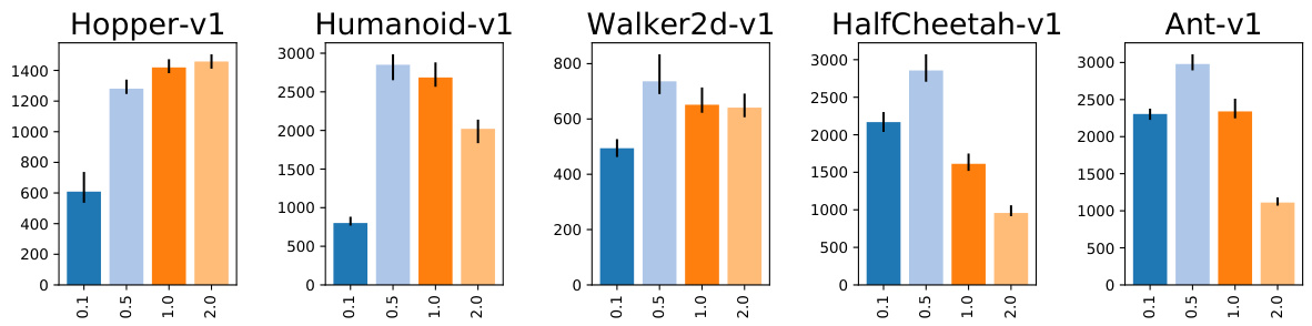
Figure 2: Comparison of different initial standard deviations of actions (C61).
图 2: 不同动作初始标准差对比 (C61)。
Fig. 17 compares two approaches to transform unbounded sampled actions into the bounded $[-1,1]$ domain expected by the environment (C63): clipping and applying a tanh function. tanh performs slightly better overall (in particular it improves the performance on Half Cheetah by $30%$ ). Comparing Fig. 17 and Fig. 2 suggests that the difference might be mostly caused by the decreased magnitude of initial actions9.
图 17 比较了两种将无界采样动作转换为环境 (C63) 预期的有界 $[-1,1]$ 区间的方法:截断 (clipping) 和应用 tanh 函数。总体而言 tanh 表现略优 (特别是它在 Half Cheetah 任务上将性能提升了 $30%$)。对比图 17 和图 2 可知,这种差异可能主要由初始动作幅度的降低所导致[9]。
Other choices appear to be less important: The scale of the last layer initialization matters much less for the value MLP (C58) than for the policy MLP (Fig. 19). Apart from the last layer scaling, the network initialization scheme (C56) does not matter too much (Fig. 27). Only he_normal and he_uniform [7] appear to be suboptimal choices with the other options performing very similarly. There also appears to be no clear benefits if the standard deviation of the policy is learned for each state (i.e. outputted by the policy network) or once globally for all states (C59, Fig. 23). For the transformation of policy output into action standard deviation (C60), softplus and exponentiation perform very similarly 10 (Fig. 25). Finally, the minimum action standard deviation (C62) seems to matter little, if it is not set too large (Fig. 30).
其他选择似乎不太重要:最后一层初始化的规模对值MLP (C58) 的影响远小于对策略MLP (图19) 的影响。除了最后一层缩放外,网络初始化方案 (C56) 的影响也不大 (图27)。只有he_normal和he_uniform [7] 表现稍逊,其他选项的效果非常接近。此外,无论是为每个状态单独学习策略的标准差 (即由策略网络输出) 还是全局统一学习 (C59, 图23),似乎都没有明显优势。在将策略输出转换为动作标准差时 (C60),softplus和指数变换的效果非常相似 (图25)。最后,只要不设置得过大,最小动作标准差 (C62) 的影响似乎很小 (图30)。
Recommendation. Initialize the last policy layer with $100\times$ smaller weights. Use softplus to transform network output into action standard deviation and add a (negative) offset to its input to decrease the initial standard deviation of actions. Tune this offset if possible. Use tanh both as the activation function (if the networks are not too deep) and to transform the samples from the normal distribution to the bounded action space. Use a wide value MLP (no layers shared with the policy) but tune the policy width (it might need to be narrower than the value MLP).
建议:将最后一层策略网络的权重初始化为原值的1/100。使用softplus函数将网络输出转换为动作标准差,并在其输入中添加负偏移量以降低动作的初始标准差。如有可能,请调整此偏移量。若网络深度适中,可同时采用tanh作为激活函数,并将正态分布样本转换至有界动作空间。使用宽度较大的价值网络MLP(不与策略网络共享层),但需调整策略网络宽度(可能需比价值网络MLP更窄)。
3.3 Normalization and clipping (based on the results in Appendix F)
3.3 归一化与剪枝 (基于附录F中的结果)
Study description. We investigate the impact of different normalization techniques: observation normalization (C64), value function normalization (C66), per-minibatch advantage normalization (C67), as well as gradient (C68) and observation (C65) clipping.
研究描述。我们研究了不同归一化技术的影响:观测归一化 (C64)、价值函数归一化 (C66)、每小批量优势归一化 (C67),以及梯度裁剪 (C68) 和观测裁剪 (C65)。
Interpretation. Input normalization (C64) is crucial for good performance on all environments apart from Hopper (Fig. 33). Quite surprisingly, value function normalization (C66) also influences the performance very strongly — it is crucial for good performance on Half Cheetah and Humanoid, helps slightly on Hopper and Ant and significantly hurts the performance on Walker2d (Fig. 37). We are not sure why the value function scale matters that much but suspect that it affects the performance by changing the speed of the value function fitting.11 In contrast to observation and value function normalization, per-minibatch advantage normalization (C67) seems not to affect the performance too much (Fig. 35). Similarly, we have found little evidence that clipping normalized 12 observations (C65) helps (Fig. 38) but it might be worth using if there is a risk of extremely high observations due to simulator divergence. Finally, gradient clipping (C68) provides a small performance boost with the exact clipping threshold making little difference (Fig. 34).
解读。输入归一化(C64)对所有环境下的性能都至关重要,除了Hopper(图33)。令人惊讶的是,价值函数归一化(C66)对性能也有很强的影响——它对Half Cheetah和Humanoid的良好性能至关重要,对Hopper和Ant略有帮助,但会显著降低Walker2d的性能(图37)。我们不确定为什么价值函数尺度如此重要,但怀疑它通过改变价值函数拟合的速度来影响性能。与观测值和价值函数归一化相比,每小批量优势归一化(C67)似乎对性能影响不大(图35)。同样,我们发现几乎没有证据表明裁剪归一化观测值(C65)有帮助(图38),但如果由于模拟器发散而存在极高观测值的风险,可能值得使用。最后,梯度裁剪(C68)提供了小幅性能提升,而具体的裁剪阈值几乎没有影响(图34)。
Recommendation. Always use observation normalization and check if value function normalization improves performance. Gradient clipping might slightly help but is of secondary importance.
建议:始终使用观测归一化,并检查值函数归一化是否能提升性能。梯度裁剪可能略有帮助,但属于次要优化手段。
3.4 Advantage Estimation (based on the results in Appendix G)
3.4 优势估计 (基于附录G的结果)
Study description. We compare the most commonly used advantage estimators (C6): N-step [3], GAE [9] and V-trace [19] and their hyper parameters (C7, C8, C9, C10). We also experiment with applying PPO-style pessimistic clipping (C13) to the value loss (present in the original PPO implementation but not mentioned in the PPO paper [17]) and using Huber loss [1] instead of MSE for value learning (C11, C12). Moreover, we varied the number of parallel environments used (C1) as it changes the length of the experience fragments collected in each step.
研究描述。我们比较了最常用的优势估计器 (C6):N步 [3]、GAE [9] 和 V-trace [19] 及其超参数 (C7、C8、C9、C10)。我们还尝试将 PPO 风格的悲观剪裁 (C13) 应用于价值损失(原始 PPO 实现中存在但未在 PPO 论文 [17] 中提及),并使用 Huber 损失 [1] 代替 MSE 进行价值学习 (C11、C12)。此外,我们改变了使用的并行环境数量 (C1),因为它会改变每一步收集的经验片段的长度。
Interpretation. GAE and V-trace appear to perform better than N-step returns (Fig. 44 and 40) which indicates that it is beneficial to combine the value estimators from multiple timesteps. We have not found a significant performance difference between GAE and V-trace in our experiments. $\lambda=0.9$ (C8, C9) performed well regardless of whether GAE (Fig. 45) or V-trace (Fig. 49) was used on all tasks but tuning this value per environment may lead to modest performance gains. We have found that PPO-style value loss clipping (C13) hurts the performance regardless of the clipping threshold 13 (Fig. 43). Similarly, the Huber loss (C11) performed worse than MSE in all environments (Fig. 42) regardless of the value of the threshold (C12) used (Fig. 48).
解读。GAE和V-trace的表现似乎优于N步回报(图44和40),这表明结合多个时间步长的价值估计器是有益的。在我们的实验中,未发现GAE与V-trace存在显著性能差异。$\lambda=0.9$(C8, C9)在所有任务中表现良好,无论使用GAE(图45)还是V-trace(图49),但针对不同环境调整该值可能带来小幅性能提升。我们发现PPO风格的价值损失裁剪(C13)会损害性能,且与裁剪阈值13无关(图43)。类似地,在所有环境中Huber损失(C11)的表现均逊于MSE(图42),且与所用阈值(C12)的值无关(图48)。
Recommendation. Use GAE with $\lambda=0.9$ but neither Huber loss nor PPO-style value loss clipping.
建议:使用GAE (Generalized Advantage Estimation) 并设置$\lambda=0.9$,但不要使用Huber损失函数或PPO风格的值损失裁剪。
3.5 Training setup (based on the results in Appendix H)
3.5 训练设置 (基于附录H中的结果)
Study description. We investigate choices related to the data collection and minibatch handling: the number of parallel environments used (C1), the number of transitions gathered in each iteration (C2), the number of passes over the data (C3), minibatch size (C4) and how the data is split into mini batches (C5).
研究描述。我们调查了与数据收集和小批量处理相关的选择:使用的并行环境数量 (C1)、每次迭代收集的转移数量 (C2)、数据遍历次数 (C3)、小批量大小 (C4) 以及数据如何分割成小批量 (C5)。
For the last choice, in addition to standard choices, we also consider a new small modification of the original PPO approach: The original PPO implementation splits the data in each policy iteration step into individual transitions and then randomly assigns them to mini batches (C5). This makes it impossible to compute advantages as the temporal structure is broken. Therefore, the advantages are computed once at the beginning of each policy iteration step and then used in minibatch policy and value function optimization. This results in higher diversity of data in each minibatch at the cost of using slightly stale advantage estimations. As a remedy to this problem, we propose to recompute the advantages at the beginning of each pass over the data instead of just once per iteration.
对于最后一种选择,除了标准选项外,我们还考虑对原始PPO方法进行一个小改动:原始PPO实现在每次策略迭代步骤中将数据拆分为独立转移样本,然后随机分配到小批次中(C5)。这种做法由于破坏了时序结构而无法计算优势函数。因此,优势值会在每次策略迭代步骤开始时统一计算,随后用于小批次的策略和价值函数优化。这虽然提高了每个小批次的数据多样性,但代价是使用了略微过时的优势估计。针对该问题,我们提出在每次数据遍历开始时重新计算优势值,而非仅在每个迭代步骤计算一次。
Results. Un surprisingly, going over the experience multiple times appears to be crucial for good sample complexity (Fig. 54). Often, this is computationally cheap due to the simple models considered, in particular on machines with accelerators such as GPUs and TPUs. As we increase the number of parallel environments (C1), performance decreases sharply on some of the environments (Fig. 55). This is likely caused by shortened experience chunks (See Sec. B.1 for the detailed description of the data collection process) and earlier value boots trapping. Despite that, training with more environments usually leads to faster training in wall-clock time if enough CPU cores are available. Increasing the batch size (C4) does not appear to hurt the sample complexity in the range we tested (Fig. 57) which suggests that it should be increased for faster iteration speed. On the other hand, the number of transitions gathered in each iteration (C2) influences the performance quite significantly (Fig. 52). Finally, we compare different ways to handle mini batches (See Sec. B.1 for the detailed description of different variants) in Fig. 53 and 58. The plots suggest that stale advantages can in fact hurt performance and that re computing them at the beginning of each pass at least partially mitigates the problem and performs best among all variants.
结果。不出所料,多次重复经验对获得良好的样本复杂度至关重要(图54)。由于所考虑的模型较为简单,这一过程通常计算成本较低,尤其是在配备GPU和TPU等加速器的机器上。当我们增加并行环境数量(C1)时,部分环境下的性能急剧下降(图55)。这可能是由于经验片段缩短(数据收集过程的详细描述见附录B.1)和早期价值引导所致。尽管如此,若有足够的CPU核心,使用更多环境进行训练通常能缩短实际训练时间。增大批次大小(C4)在我们测试范围内似乎不会损害样本复杂度(图57),这表明应增大批次以加快迭代速度。另一方面,每次迭代收集的状态转换数量(C2)对性能影响显著(图52)。最后,我们在图53和图58中比较了处理小批次的不同方法(各变体的详细描述见附录B.1)。图表表明,过期的优势值确实会损害性能,而在每次遍历开始时重新计算这些值至少能部分缓解该问题,且在所有变体中表现最佳。
Recommendation. Go over experience multiple times. Shuffle individual transitions before assigning them to mini batches and recompute advantages once per data pass (See App. B.1 for the details). For faster wall-clock time training use many parallel environments and increase the batch size (both might hurt the sample complexity). Tune the number of transitions in each iteration (C2) if possible.
建议:多次回顾经验。在将单个转换分配到小批次之前进行随机打乱,并在每次数据通过时重新计算优势值(详见附录B.1)。为缩短实际训练时间,可使用多个并行环境并增大批次大小(二者可能影响样本复杂度)。如有可能,调整每次迭代中的转换数量(C2)。
3.6 Timesteps handling (based on the results in Appendix I)
3.6 时间步处理 (基于附录I中的结果)
Study description. We investigate choices related to the handling of timesteps: discount fac $\mathrm{tor}^{14}$ (C20), frame skip (C21), and how episode termination due to timestep limits are handled (C22). The latter relates to a technical difficulty explained in App. B.4 where one assumes for the algorithm an infinite time horizon but then trains using a finite time horizon [16].
研究描述。我们调查了与时间步处理相关的选择:折扣因子 (discount factor) (C20)、帧跳过 (frame skip) (C21) 以及如何处理因时间步限制导致的回合终止 (C22)。后者涉及附录 B.4 中解释的一个技术难点,即假设算法具有无限时间范围,但实际上使用有限时间范围进行训练 [16]。
Interpretation. Fig. 60 shows that the performance depends heavily on the discount factor $\gamma$ (C20) with $\gamma=0.99$ performing reasonably well in all environments. Skipping every other frame (C21) improves the performance on 2 out of 5 environments (Fig. 61). Proper handling of episodes abandoned due to the timestep limit seems not to affect the performance (C22, Fig. 62) which is probably caused by the fact that the timestep limit is quite high (1000 transitions) in all the environments we considered.
解读。图60表明性能很大程度上取决于折扣因子$\gamma$ (C20),其中$\gamma=0.99$在所有环境中表现都相当不错。隔帧跳过(C21)在5个环境中的2个提升了性能(图61)。由于时间步限制而中断的回合似乎并未影响性能(C22,图62),这可能是因为我们所考虑的所有环境中时间步限制都较高(1000次状态转移)。
Recommendation. Discount factor $\gamma$ is one of the most important hyper parameters and should be tuned per environment (start with $\gamma=0.99,$ ). Try frame skip if possible. There is no need to handle environments step limits in a special way for large step limits.
建议。折扣因子 $\gamma$ 是最重要的超参数之一,应根据具体环境进行调整(建议从 $\gamma=0.99$ 开始)。如有可能,尝试使用帧跳过(frame skip)技术。对于步数限制较大的环境,无需特殊处理步数限制问题。
3.7 Optimizers (based on the results in Appendix J)
3.7 优化器 (基于附录J中的结果)
Study description. We investigate two gradient-based optimizers commonly used in RL: (C23) – Adam [8] and RMSprop – as well as their hyper parameters (C24, C25, C26, C27, C28, C29, C30) and a linear learning rate decay schedule (C31).
研究描述。我们研究了两种强化学习中常用的基于梯度的优化器:(C23) – Adam [8] 和 RMSprop,以及它们的超参数 (C24、C25、C26、C27、C28、C29、C30) 和线性学习率衰减调度 (C31)。
Interpretation. The differences in performance between the optimizers (C23) appear to be rather small with no optimizer consistently outperforming the other across environments (Fig. 66). Unsurprisingly, the learning rate influences the performance very strongly (Fig. 69) with the default value of 0.0003 for Adam (C24) performing well on all tasks. Fig. 67 shows that Adam works better with momentum (C26). For RMSprop, momentum (C27) makes less difference (Fig. 71) but our results suggest that it might slightly improve performance 15. Whether the centered or uncentered version of RMSprop is used (C30) makes no difference (Fig. 70) and similarly we did not find any difference between different values of the $\epsilon$ coefficients (C28, C29, Fig. 68 and 72). Linearly decaying the learning rate to 0 increases the performance on 4 out of 5 tasks but the gains are very small apart from Ant, where it leads to $15%$ higher scores (Fig. 65).
解读。不同优化器 (C23) 之间的性能差异似乎相当小,没有哪种优化器在所有环境中持续优于其他优化器 (图 66)。不出所料,学习率对性能影响很大 (图 69),Adam (C24) 的默认值 0.0003 在所有任务上都表现良好。图 67 显示 Adam 配合动量 (C26) 效果更好。对于 RMSprop,动量 (C27) 的影响较小 (图 71),但我们的结果表明它可能会略微提升性能 15。使用 RMSprop 的中心化或非中心化版本 (C30) 没有差异 (图 70),同样我们发现 $\epsilon$ 系数 (C28, C29, 图 68 和 72) 的不同取值之间也没有任何差异。将学习率线性衰减至 0 可以提升 5 个任务中 4 个的性能,但除了 Ant 任务 (分数提高了 $15%$) 外,其他增益都非常小 (图 65)。
Recommendation. Use Adam [8] optimizer with momentum $\beta_{1}=0.9$ and a tuned learning rate (0.0003 is a safe default). Linearly decaying the learning rate may slightly improve performance but is of secondary importance.
建议:使用带有动量 $\beta_{1}=0.9$ 的Adam [8]优化器,并调整学习率(0.0003是安全的默认值)。线性衰减学习率可能略微提升性能,但属于次要因素。
3.8 Regular iz ation (based on the results in Appendix K)
3.8 正则化 (基于附录K的结果)
Study description. We investigate different policy regularize rs (C32), which can have either the form of a penalty (C33, e.g. bonus for higher entropy) or a soft constraint (C34, e.g. entropy should not be lower than some threshold) which is enforced with a Lagrange multiplier. In particular, we consider the following regular iz ation terms: entropy (C40, C46), the Kullback–Leibler divergence (KL) between a reference $\mathcal{N}(0,1)$ action distribution and the current policy (C37, C43) and the KL divergence and reverse KL divergence between the current policy and the behavioral one (C35, C41, C36, C42), as well as the “decoupled” KL divergence from [18, 34] (C38, C39, C44, C45).
研究描述。我们研究了不同的策略正则化器 (C32),其形式可以是惩罚项 (C33,例如对更高熵的奖励) 或通过拉格朗日乘数强制实施的软约束 (C34,例如熵不应低于某个阈值)。具体而言,我们考虑了以下正则化项:熵 (C40, C46)、参考动作分布 $\mathcal{N}(0,1)$ 与当前策略之间的Kullback-Leibler散度 (KL) (C37, C43)、当前策略与行为策略之间的KL散度及逆KL散度 (C35, C41, C36, C42),以及来自[18, 34]的"解耦"KL散度 (C38, C39, C44, C45)。
Interpretation. We do not find evidence that any of the investigated regularize rs helps significantly on our environments with the exception of Half Cheetah on which all constraints (especially the entropy constraint) help (Fig. 76 and 77). However, the performance boost is largely independent on the constraint threshold (Fig. 83, 84, 87, 89, 90 and 91) which suggests that the effect is caused by the initial high strength of the penalty (before it gets adjusted) and not by the desired constraint. While it is a bit surprising that regular iz ation does not help at all (apart from Half Cheetah), we conjecture that regular iz ation might be less important in our experiments because: (1) the PPO policy loss already enforces the trust region which makes KL penalties or constraints redundant; and (2) the careful policy initialization (See Sec. 3.2) is enough to guarantee good exploration and makes the entropy bonus or constraint redundant.
解释。我们没有发现证据表明所研究的任何正则化方法在除Half Cheetah外的环境中能显著提升性能 (图76和77) 。然而,性能提升在很大程度上与约束阈值无关 (图83、84、87、89、90和91) ,这表明效果是由惩罚初始高强度 (在调整前) 而非预期约束引起的。虽然正则化完全无效 (除Half Cheetah外) 有些令人意外,但我们推测正则化在实验中可能不太重要,因为:(1) PPO策略损失已强制执行信任区域,使得KL惩罚或约束变得冗余;(2) 谨慎的策略初始化 (参见第3.2节) 足以保证良好的探索,使得熵奖励或约束变得冗余。
4 Related Work
4 相关工作
Islam et al. [15] and Henderson et al. [22] point out the reproducibility issues in RL including the performance differences between different code bases, the importance of hyper parameter tuning and the high level of stochastic it y due to random seeds. Tucker et al. [26] showed that the gains, which had been attributed to one of the recently proposed policy gradients improvements, were, in fact, caused by the implementation details. The most closely related work to ours is probably Engstrom et al. [27] where the authors investigate code-level improvements in the PPO [17] code base and conclude that they are responsible for the most of the performance difference between PPO and TRPO [10]. Our work is also similar to other large-scale studies done in other fields of Deep Learning, e.g. model-based RL [31], GANs [24], NLP [35], disentangled representations [23] and convolution network architectures [36].
Islam等[15]和Henderson等[22]指出了强化学习(RL)中的可复现性问题,包括不同代码库间的性能差异、超参数调优的重要性以及随机种子导致的高度随机性。Tucker等[26]证明,曾被归因于近期某策略梯度改进方案的性能提升,实际上是由实现细节引起的。与我们研究最相关的工作可能是Engstrom等[27],作者通过研究PPO[17]代码库的代码级改进,得出结论认为这些改进是造成PPO与TRPO[10]性能差异的主要原因。我们的工作也类似于深度学习其他领域开展的大规模研究,例如基于模型的强化学习[31]、GAN[24]、自然语言处理(NLP)[35]、解耦表示[23]和卷积网络架构[36]。
5 Conclusions
5 结论
In this paper, we investigated the importance of a broad set of high- and low-level choices that need to be made when designing and implementing on-policy learning algorithms. Based on more than $250^{\ '}000$ experiments in five continuous control environments, we evaluate the impact of different choices and provide practical recommendations. One of the surprising insights is that the initial action distribution plays an important role in agent performance. We expect this to be a fruitful avenue for future research.
在本文中,我们研究了设计和实现同策略(on-policy)学习算法时需要做出的一系列高层次和低层次选择的重要性。基于在五个连续控制环境中进行的超过$250^{\ '}000$次实验,我们评估了不同选择的影响并提供了实用建议。其中一个令人惊讶的发现是初始动作分布对智能体性能具有重要影响。我们预计这将成为未来研究的一个富有成果的方向。
References
参考文献
A Reinforcement Learning Background
强化学习背景
We consider the standard reinforcement learning formalism consisting of an agent interacting with an environment. To simplify the exposition we assume in this section that the environment is fully observable. An environment is described by a set of states $s$ , a set of actions $\mathcal{A}$ , a distribution of initial states $p(s_{0})$ , a reward function $r:S\times A\to\mathbb{R}$ , transition probabilities $p(s_{t+1}|s_{t},a_{t})$ $t$ is a timestep index explained later), termination probabilities $T(s_{t},a_{t})$ and a discount factor $\gamma\in[0,1]$ .
我们考虑标准的强化学习框架,即智能体与环境交互的形式。为简化说明,本节假设环境是完全可观测的。环境由以下要素描述:状态集合 $s$、动作集合 $\mathcal{A}$、初始状态分布 $p(s_{0})$、奖励函数 $r:S\times A\to\mathbb{R}$、转移概率 $p(s_{t+1}|s_{t},a_{t})$ (其中 $t$ 是稍后解释的时间步索引)、终止概率 $T(s_{t},a_{t})$ 以及折扣因子 $\gamma\in[0,1]$。
A policy $\pi$ is a mapping from state to a distribution over actions. Every episode starts by sampling an initial state $s_{0}$ . At every timestep $t$ the agent produces an action based on the current state: $a_{t}\sim\pi(\cdot|s_{t})$ . In turn, the agent receives a reward $r_{t}=r(s_{t},a_{t})$ and the environment’s state is updated. With probability $T(s_{t},a_{t})$ the episode is terminated, and otherwise the new environments state $s_{t+1}$ is sampled from $p(\cdot|s_{t},a_{t})$ . The discounted sum of future rewards, also referred to as the return, is defined as $\textstyle R_{t}=\sum_{i=t}^{\infty}\gamma^{i-t}r_{i}$ . The agent’s goal is to find the policy $\pi$ which maximizes the expected return $\mathbb{E}_ {\pi}[R_{0}|s_{0}]$ , where the expectation is taken over the initial state distribution, the policy, and environment transitions accordingly to the dynamics specified above. The $Q$ -function or action-value function of a given policy $\pi$ is defined as $Q^{\pi}(s_{t},a_{t})=\mathbb{E}_ {\pi}[R_{t}|\bar{s}_ {t},a_{t}]$ , while the V-function or state-value function is defined as $V^{\pi}(s_{t})=\mathbb{E}_ {\pi}[R_{t}|s_{t}]$ . The value $A^{\pi}(s_{t},a_{t})=Q^{\pi}(s_{t},a_{t})-V^{\pi}(s_{t})$ is called the advantage and tells whether the action $a_{t}$ is better or worse than an average action the policy $\pi$ takes in the state $s_{t}$ .
策略 $\pi$ 是从状态到动作分布的映射。每个回合从采样初始状态 $s_{0}$ 开始。在每一步时间 $t$,智能体根据当前状态生成动作:$a_{t}\sim\pi(\cdot|s_{t})$。随后,智能体获得奖励 $r_{t}=r(s_{t},a_{t})$,环境状态随之更新。以概率 $T(s_{t},a_{t})$ 终止回合,否则从 $p(\cdot|s_{t},a_{t})$ 采样新环境状态 $s_{t+1}$。未来奖励的折现总和(即回报)定义为 $\textstyle R_{t}=\sum_{i=t}^{\infty}\gamma^{i-t}r_{i}$。智能体的目标是找到最大化期望回报 $\mathbb{E}_ {\pi}[R_{0}|s_{0}]$ 的策略 $\pi$,其中期望值基于初始状态分布、策略及符合上述动态的环境转移计算。给定策略 $\pi$ 的 $Q$ 函数(动作价值函数)定义为 $Q^{\pi}(s_{t},a_{t})=\mathbb{E}_{\pi}[R_{t}|\bar{s}_ {t},a_{t}]$,而 $V$ 函数(状态价值函数)定义为 $V^{\pi}(s_{t})=\mathbb{E}_ {\pi}[R_{t}|s_{t}]$。值 $A^{\pi}(s_{t},a_{t})=Q^{\pi}(s_{t},a_{t})-V^{\pi}(s_{t})$ 称为优势函数,用于判断动作 $a_{t}$ 优于或劣于策略 $\pi$ 在状态 $s_{t}$ 下的平均动作。
In practice, the policies and value functions are going to be represented as neural networks. In particular, RL algorithms we consider maintain two neural networks: one representing the current policy $\pi$ and a value network which approximates the value function of the current policy $V\approx V^{\pi}$ .
在实践中,策略和价值函数将用神经网络表示。具体而言,我们考虑的强化学习算法会维护两个神经网络:一个表示当前策略 $\pi$,另一个是价值网络,用于近似当前策略的价值函数 $V\approx V^{\pi}$。
B List of Investigated Choices
B 调研选项列表
In this section we list all algorithmic choices which we consider in our experiments. See Sec. A for a very brief introduction to RL and the notation we use in this section.
在本节中,我们列出了实验中考虑的所有算法选择。关于强化学习(RL)的简要介绍及本节使用的符号说明,请参阅附录A。
B.1 Data collection and optimization loop
B.1 数据收集与优化循环
RL algorithms interleave running the current policy in the environment with policy and value function networks optimization. In particular, we create num_envs (C1) environments [14]. In each iteration, we run all environments synchronously sampling actions from the current policy until we have gathered iteration size (C2) transitions total (this means that we have num_envs (C1) experience fragments, each consisting of iteration size (C2) / num_envs (C1) transitions). Then, we perform num_epochs (C3) epochs of minibatch updates where in each epoch we split the data into mini batches of size batch_size (C4), and performing gradient-based optimization [17]. Going over collected experience multiple times means that it is not strictly an on-policy RL algorithm but it may increase the sample complexity of the algorithm at the cost of more computationally expensive optimization step.
强化学习(RL)算法通过在环境中交替执行当前策略与策略及价值函数网络优化来实现训练。具体而言,我们会创建num_envs (C1)个环境[14]。在每次迭代中,我们同步运行所有环境并从当前策略中采样动作,直到总共收集到iteration_size (C2)个状态转换(这意味着我们将获得num_envs (C1)段经验片段,每段包含iteration_size (C2)/num_envs (C1)个转换)。随后,我们进行num_epochs (C3)轮小批量更新,每轮将数据划分为batch_size (C4)大小的小批量,并执行基于梯度的优化[17]。对收集的经验进行多次遍历意味着这并非严格的在线策略RL算法,但可能会以更高计算成本的优化步骤为代价,提高算法的样本复杂度。
We consider four different variants of the above scheme (choice C5):
我们考虑上述方案的四种不同变体(选择 C5):
B.2 Advantage estimation
B.2 优势估计
Let $V$ be an approx im at or of the value function of some policy, i.e. $V\approx V^{\pi}$ . We experimented with the three most commonly used advantage estimators in on-policy RL (choice C6):
设 $V$ 为某策略价值函数的近似值,即 $V\approx V^{\pi}$。我们测试了在线策略强化学习中最常用的三种优势估计器(选择 C6):
• N-step return [3] is defined as
• N步回报 (N-step return) [3] 定义为
$$
\hat{V}_ {t}^{(N)}=\sum_{i=t}^{t+N-1}\gamma^{i-t}r_{i}+\gamma^{N}V(s_{t+N})\approx V^{\pi}(s_{t}).
$$
$$
\hat{V}_ {t}^{(N)}=\sum_{i=t}^{t+N-1}\gamma^{i-t}r_{i}+\gamma^{N}V(s_{t+N})\approx V^{\pi}(s_{t}).
$$
The parameter $N$ (choice C7) controls the bias–variance tradeoff of the estimator with bigger values resulting in an estimator closer to empirical returns and having less bias and more variance. Given N-step returns we can estimate advantages as follows:
参数 $N$ (选项 C7) 控制估计器的偏差-方差权衡,较大的值会使估计结果更接近经验回报,偏差更小而方差更大。给定 N 步回报后,我们可以按如下方式估计优势值:
$$
\hat{A}_ {t}^{\mathrm{(N)}}=\hat{V}_ {t}^{\mathrm{(N)}}-V\big(s_{t}\big)\approx A^{\pi}\big(s_{t},a_{t}\big).
$$
$$
\hat{A}_ {t}^{\mathrm{(N)}}=\hat{V}_ {t}^{\mathrm{(N)}}-V\big(s_{t}\big)\approx A^{\pi}\big(s_{t},a_{t}\big).
$$
• Generalized Advantage Estimator, $\mathbf{GAE}(\lambda)$ [9] is a method that combines multi-step returns in the following way:
• 广义优势估计器 (Generalized Advantage Estimator), $\mathbf{GAE}(\lambda)$ [9] 是一种通过以下方式组合多步回报的方法:
$$
\hat{V}_ {t}^{\mathrm{GAE}}=(1-\lambda)\sum_{N>0}\lambda^{N-1}\hat{V}_ {t}^{(N)}\approx V^{\pi}(s_{t}),
$$
$$
\hat{V}_ {t}^{\mathrm{GAE}}=(1-\lambda)\sum_{N>0}\lambda^{N-1}\hat{V}_ {t}^{(N)}\approx V^{\pi}(s_{t}),
$$
where $0<\lambda<1$ is a hyper parameter (choice C8) controlling the bias–variance trade-off. Using this, we can estimate advantages with:
其中 $0<\lambda<1$ 是控制偏差-方差权衡的超参数 (选项 C8)。利用该参数,我们可以通过以下公式估算优势:
$$
\hat{A}_ {t}^{\mathrm{GAE}}=\hat{V}_ {t}^{\mathrm{GAE}}-V(s_{t})\approx A^{\pi}(s_{t},a_{t}).
$$
$$
\hat{A}_ {t}^{\mathrm{GAE}}=\hat{V}_ {t}^{\mathrm{GAE}}-V(s_{t})\approx A^{\pi}(s_{t},a_{t}).
$$
It is possible to compute the values of this estimator for all states encountered in an episode in linear time [9].
可以在线性时间内计算该估计器在某一回合中遇到的所有状态的值 [9]。
• $\mathbf{V-trace}(\lambda,\bar{c},\bar{\rho})$ [19] is an extension of GAE which introduces truncated importance sampling weights to account for the fact that the current policy might be slightly different from the policy which generated the experience. It is parameterized by $\lambda$ (choice C9) which serves the same role as in GAE and two parameters $\bar{c}$ and $\bar{\rho}$ which are truncation thresholds for two different types of importance weights. See [19] for the detailed description of the $\mathrm{V}.$ -trace estimator. All experiments in the original paper [19] use $\bar{c}=\bar{\rho}=1$ . Similarly, we only consider the case $\bar{c}=\bar{\rho}$ , i.e., we consider a single choice $\mathtt{V}$ -Trace advantage $c$ , $\rho$ (C10).
• $\mathbf{V-trace}(\lambda,\bar{c},\bar{\rho})$ [19] 是 GAE 的扩展,通过引入截断重要性采样权重来解决当前策略可能与生成经验数据的策略略有差异的问题。该算法由 $\lambda$ (选项 C9)参数化(其作用与 GAE 中的相同),以及两个截断阈值参数 $\bar{c}$ 和 $\bar{\rho}$ (用于两类不同的重要性权重)。关于 V-trace 估计器的详细说明请参阅 [19]。原论文 [19] 的所有实验均采用 $\bar{c}=\bar{\rho}=1$。类似地,我们仅考虑 $\bar{c}=\bar{\rho}$ 的情况,即设定单一选项 $\mathtt{V}$-Trace 优势参数 $c$, $\rho$ (C10)。
The value network is trained by fitting one of the returns described above with an MSE (quadratic) or a Huber [1] loss (choice C11). Huber loss is a quadratic around zero up to some threshold (choice C12) at which point it becomes a linear function.
价值网络通过用均方误差 (MSE) 或 Huber [1] 损失 (选项 C11) 拟合上述任一回报进行训练。Huber 损失在零点附近呈二次函数,直至达到某个阈值 (选项 C12) 后转变为线性函数。
The original PPO implementation [17] uses an additional pessimistic clipping in the value loss function. See [27] for the description of this technique. It is parameterized by a clipping threshold (choice C13).
原始PPO实现[17]在价值损失函数中使用了额外的悲观剪枝技术。该方法的详细说明参见[27],其通过剪枝阈值(choice C13)进行参数化。
B.3 Policy losses
B.3 策略损失
Let $\pi$ denote the policy being optimized, and $\mu$ the behavioral policy, i.e. the policy which generated the experience. Moreover, let $\hat{A}_ {t}^{\pi}$ and $\hat{A}_{t}^{\mu}$ be some estimators of the advantage at timestep $t$ for the policies $\pi$ and $\mu$
设 $\pi$ 表示待优化的策略,$\mu$ 表示行为策略 (behavioral policy),即生成经验数据的策略。此外,令 $\hat{A}_ {t}^{\pi}$ 和 $\hat{A}_{t}^{\mu}$ 分别表示策略 $\pi$ 和 $\mu$ 在时间步 $t$ 的优势估计量。
We consider optimizing the policy with the following policy losses (choice C14):
我们考虑用以下策略损失来优化策略(选项 C14):
Policy Gradients (PG) [2] with advantages: $\mathcal{L}_ {\mathtt{P G}}=-\log\pi(a_{t}|s_{t})\hat{A}_ {t}^{\pi}$ . It can be shown that if $\hat{A}_ {t}^{\pi}$ estimators are unbiased, then $\nabla_{\boldsymbol{\theta}}\mathcal{L}_ {\mathtt{P G}}$ is an unbiased estimator of the gradient of the policy performance assuming that experience was generated by the current policy $\pi$ . • V-trace [19]: $\mathcal{L}_ {\mathtt{V\mathrm{-trace}}}^{\bar{\rho}}=\mathbf{sg}(\rho_{t})\mathcal{L}_ {\mathtt{P G}}$ , where $\begin{array}{r}{\rho_{t}=\operatorname*{min}(\frac{\pi(a_{t}|s_{t})}{\mu(a_{t}|s_{t})},\bar{\rho})}\end{array}$ is a truncated importance weight, sg is the stop gradient operator17 and $\bar{\rho}$ is a hyper parameter (choice C15). $\nabla_{\theta}L_{\mathtt{V-t r a c e}}^{\bar{\rho}}$ is an un18biased estimator of the gradient of the policy performance if $\bar{\rho}=\infty$ regardless of the behavioural policy $\mu^{18}$ .
策略梯度 (Policy Gradients, PG) [2] 带优势函数: $\mathcal{L}_ {\mathtt{P G}}=-\log\pi(a_{t}|s_{t})\hat{A}_ {t}^{\pi}$。可以证明,若 $\hat{A}_ {t}^{\pi}$ 估计量是无偏的,则当经验数据由当前策略 $\pi$ 生成时,$\nabla_{\boldsymbol{\theta}}\mathcal{L}_{\mathtt{P G}}$ 是策略性能梯度的无偏估计量。
• V-trace [19]: $\mathcal{L}_ {\mathtt{V\mathrm{-trace}}}^{\bar{\rho}}=\mathbf{sg}(\rho_{t})\mathcal{L}_ {\mathtt{P G}}$,其中 $\begin{array}{r}{\rho_{t}=\operatorname*{min}(\frac{\pi(a_{t}|s_{t})}{\mu(a_{t}|s_{t})},\bar{\rho})}\end{array}$ 为截断重要性权重,sg表示梯度停止算子,$\bar{\rho}$ 为超参数 (选择 C15)。当 $\bar{\rho}=\infty$ 时,无论行为策略 $\mu^{18}$ 如何,$\nabla_{\theta}L_{\mathtt{V-t r a c e}}^{\bar{\rho}}$ 都是策略性能梯度的无偏估计量。
• Proximal Policy Optimization (PPO) [17]:
• 近端策略优化 (PPO) [17]:
$$
\mathcal L_{\mathrm{PP0}}^{\epsilon}=-\operatorname*{min}\left[\frac{\pi(a_{t}|s_{t})}{\mu(a_{t}|s_{t})}\hat{A}_ {t}^{\pi},\mathrm{clip}\left(\frac{\pi(a_{t}|s_{t})}{\mu(a_{t}|s_{t})},\frac{1}{1+\epsilon},1+\epsilon\right)\hat{A}_{t}^{\pi}\right],
$$
$$
\mathcal L_{\mathrm{PP0}}^{\epsilon}=-\operatorname*{min}\left[\frac{\pi(a_{t}|s_{t})}{\mu(a_{t}|s_{t})}\hat{A}_ {t}^{\pi},\mathrm{clip}\left(\frac{\pi(a_{t}|s_{t})}{\mu(a_{t}|s_{t})},\frac{1}{1+\epsilon},1+\epsilon\right)\hat{A}_{t}^{\pi}\right],
$$
where $\epsilon$ is a hyper parameter 19 C16. This loss encourages the policy to take actions which are better than average (have positive advantage) while clipping discourages bigger changes to the policy by limiting how much can be gained by changing the policy on a particular data point.
其中 $\epsilon$ 是一个超参数 [19 C16]。该损失函数鼓励策略采取优于平均水平(具有正优势)的动作,同时通过限制在特定数据点上改变策略所能获得的收益来抑制对策略的较大改动。
• Advantage-Weighted Regression (AWR) [33]:
• 优势加权回归 (Advantage-Weighted Regression, AWR) [33]:
$$
\mathcal{L}_ {{\mathtt{A}}{\mathtt{M}}{\mathtt{R}}}^{\beta,\omega_{\mathtt{m a x}}}=-\log\pi(a_{t}|s_{t})\operatorname*{min}\left(\exp(A_{t}^{\mu}/\beta),\omega_{\mathtt{m a x}}\right).
$$
$$
\mathcal{L}_ {{\mathtt{A}}{\mathtt{M}}{\mathtt{R}}}^{\beta,\omega_{\mathtt{m a x}}}=-\log\pi(a_{t}|s_{t})\operatorname*{min}\left(\exp(A_{t}^{\mu}/\beta),\omega_{\mathtt{m a x}}\right).
$$
It can be shown that for $\omega_{\mathrm{max}}=\infty$ (choice C17) it corresponds to an approximate optimization of the policy $\pi$ under a constraint of the form $\mathrm{KL}(\pi||\mu)<\epsilon$ where the KL bound $\epsilon$ depends on the exponentiation temperature $\beta$ (choice C18). Notice that in contrast to previous policy losses, AWR uses estimates of the advantages for the behavioral policy $(A_{t}^{\mu})$ and not the current one $(A_{t}^{\pi})$ . AWR was proposed mostly as an off-policy RL algorithm.
可以证明,当 $\omega_{\mathrm{max}}=\infty$ (选项 C17) 时,它对应于在形式为 $\mathrm{KL}(\pi||\mu)<\epsilon$ 的约束下对策略 $\pi$ 进行近似优化,其中 KL 边界 $\epsilon$ 取决于指数温度 $\beta$ (选项 C18)。需要注意的是,与之前的策略损失不同,AWR 使用行为策略 $(A_{t}^{\mu})$ 而非当前策略 $(A_{t}^{\pi})$ 的优势估计。AWR 主要被提出作为一种离策略强化学习算法。
• On-Policy Maximum a Posteriori Policy Optimization (V-MPO) [34]: This policy loss is the same as AWR with the following differences: (1) exponentiation is replaced with the softmax operator and there is no clipping with $\omega_{\mathrm{max}}$ ; (2) only samples with the top half advantages in each batch are used; (3) the temperature $\beta$ is treated as a Lagrange multiplier and adjusted automatically to keep a constraint on how much the weights (i.e. softmax outputs) diverge from a uniform distribution with the constraint threshold $\epsilon$ being a hyper parameter (choice C19). (4) A soft constraint on $\mathtt{K L}(\mu||\pi)$ is added. In our experiments, we did not treat this constraint as a part of the V-MPO policy loss as policy regular iz ation is considered separately (See Sec. B.6).
• 在线最大后验策略优化 (V-MPO) [34]:该策略损失与AWR相同,但存在以下差异:(1) 指数运算替换为softmax算子且不进行$\omega_{\mathrm{max}}$截断;(2) 仅使用每批次中优势值排名前50%的样本;(3) 将温度系数$\beta$作为拉格朗日乘子自动调整,以保持权重(即softmax输出)与均匀分布的偏离程度不超过超参数$\epsilon$设定的约束阈值(选择C19);(4) 添加对$\mathtt{K L}(\mu||\pi)$的软约束。实验中我们未将该约束纳入V-MPO策略损失,因策略正则化已单独处理(参见附录B.6节)。
• Repeat Positive Advantages (RPA): $\mathcal{L}_ {\mathtt{R P A}}=-\log\pi(a_{t}|s_{t})[A_{t}>0]^{20}$ . This is a new loss we introduce in tchoins v pear g pees r. toW ftohri eacnadu sfeo ri lVi-mMitPinOg ccoansve eorfg eAs tWo RR aPnAd wVi-thM a r re tip clu al caer,d $\mathcal{L}_ {\mathtt{A W R}}^{\beta,\omega_{\mathtt{m a x}}}$ $\omega_{\mathrm{max}}\mathcal{L}_ {\mathtt{R P A}}$ $\beta\to0$ $\epsilon\to0$ $\left[A_{t}>\bar{0}\right]$ taking the top half advantages in each batch21 (the two conditions become even more similar if advantage normalization is used, See Sec. B.9).
• 重复正向优势 (RPA): $\mathcal{L}_ {\mathtt{R P A}}=-\log\pi(a_{t}|s_{t})[A_{t}>0]^{20}$。这是我们在tchoins v pear g pees r中引入的新损失函数,用于确保Vi-MPO算法在AWR和Vi-MPO两种情况下都能收敛。通过引入$\mathcal{L}_ {\mathtt{A W R}}^{\beta,\omega_{\mathtt{m a x}}}$、$\omega_{\mathrm{max}}\mathcal{L}_ {\mathtt{R P A}}$,当$\beta\to0$且$\epsilon\to0$时,$\left[A_{t}>\bar{0}\right]$会选取每批次中排名前一半的优势值21(若使用优势归一化,这两个条件会变得更加相似,详见附录B.9)。
B.4 Handling of timesteps
B.4 时间步处理
The most important hyper parameter controlling how timesteps are handled is the discount factor $\gamma$ (choice C20). Moreover, we consider the so-called frame $s\check{k}i p^{22}$ (choice C21). Frame skip equal to $n$ means that we modify the environment by repeating each action outputted by the policy $n$ times (unless the episode has terminated in the meantime) and sum the received rewards. When using frame skip, we also adjust the discount factor appropriately, i.e. we discount with $\gamma^{n}$ instead of $\gamma$ .
控制时间步处理方式的最重要超参数是折扣因子 $\gamma$ (选项 C20)。此外,我们考虑所谓的帧跳过 $s\check{k}i p^{22}$ (选项 C21)。当帧跳过值设为 $n$ 时,意味着我们通过将策略输出的每个动作重复执行 $n$ 次(除非回合在此期间终止)并累加获得的奖励来修改环境。使用帧跳过时,我们也会相应调整折扣因子,即用 $\gamma^{n}$ 替代 $\gamma$ 进行折扣计算。
Many reinforcement learning environments (including the ones we use in our experiments) have step limits which means that an episode is terminated after some fixed number of steps (assuming it was not terminated earlier for some other reason). Moreover, the number of remaining environment steps is not included in policy observations which makes the environments non-Markovian and can potentially make learning harder [16]. We consider two ways to handle such abandoned episodes. We either treat the final transition as any other terminal transition, e.g. the value target for the last state is equal to the final reward, or we take the fact that we do not know what would happen if the episode was not terminated into account. In the latter case, we set the advantage for the final state to zero and its value target to the current value function. This also influences the value targets for prior states as the value targets are computed recursively [9, 19]. We denote this choice by Handle abandoned? (C22).
许多强化学习环境(包括我们实验中使用的那些)都设有步数限制,这意味着一个回合在达到固定步数后会终止(假设没有因其他原因提前终止)。此外,策略观察中不包含剩余环境步数,这使得环境不具备马尔可夫性,并可能增加学习难度[16]。我们考虑两种处理此类被中断回合的方法:要么将最终转换视为普通终止转换(例如最后一个状态的价值目标等于最终奖励),要么考虑我们不知道回合未被终止时会发生什么情况。在后一种情况下,我们将最终状态的优势值设为零,并将其价值目标设为当前价值函数。这还会递归影响先前状态的价值目标[9,19]。我们将这一选择标记为"处理中断?(C22)"。
B.5 Optimizers
B.5 优化器
We experiment with two most commonly used gradient-based optimizers in RL (choice C23): Adam [8] and RMSProp.23 You can find the description of the optimizers and their hyper parameters in the original publications. For both optimizers, we sweep the learning rate (choices C24 and C25), momentum (choices C26 and C27) and the $\epsilon$ parameters added for numerical stability (choice C28 and C29). Moreover, for RMSProp we consider both centered and uncentered versions (choice C30). For their remaining hyper parameters, we use the default values from TensorFlow [11], i.e. $\beta_{2}=0.999$ for Adam and $\rho=0.1$ for RMSProp. Finally, we allow a linear learning rate schedule via the hyper parameter Learning rate decay (C31) which defines the terminal learning rate as a fraction of the initial learning rate (i.e., 0.0 correspond to a decay to zero whereas 1.0 corresponds to no decay).
我们实验了强化学习中两种最常用的基于梯度的优化器(选项C23):Adam [8] 和 RMSProp。优化器及其超参数的描述可在原始文献中找到。对于这两种优化器,我们分别扫描了学习率(选项C24和C25)、动量(选项C26和C27)以及为数值稳定性添加的$\epsilon$参数(选项C28和C29)。此外,对于RMSProp,我们同时考虑了中心化和非中心化版本(选项C30)。其余超参数采用TensorFlow [11]的默认值,即Adam的$\beta_{2}=0.999$和RMSProp的$\rho=0.1$。最后,我们通过超参数"学习率衰减"(C31)启用线性学习率调度,该参数将最终学习率定义为初始学习率的比例(例如,0.0表示衰减至零,1.0表示不衰减)。
B.6 Policy regular iz ation
B.6 策略正则化
We consider three different modes for regular iz ation (choice C32):
我们考虑三种不同的正则化 (regularization) 模式 (选项 C32):
• Constraint: We impose a soft constraint of the form $R<\epsilon$ on the value of the regularize r where $\epsilon$ is a hyper parameter. This can be achieved by treating $\alpha$ as a Lagrange multiplier. In this case, we optimize the value of $\alpha>0$ together with the networks parameter by adding to the loss the term $\alpha\cdot\mathbf{sg}(\epsilon-R)$ , where sg in the stop gradient operator. In practice, we use the following para me tri z ation $\alpha=\exp(c\cdot$ $p$ ) where $p$ is a trainable parameter (initialized with 0) and $c$ is a coefficient controlling how fast $\alpha$ is adjusted (we use $c=10$ in all experiments). After each gradient step, we clip the value of $p$ to the range $[\mathrm{log}(10^{-6})/10$ , $\log(10^{6})/10]$ to avoid extremely small and large values.
• 约束: 我们对正则化项 $R$ 的值施加 $R<\epsilon$ 形式的软约束,其中 $\epsilon$ 是超参数。这可以通过将 $\alpha$ 视为拉格朗日乘数来实现。在这种情况下,我们通过在损失函数中添加 $\alpha\cdot\mathbf{sg}(\epsilon-R)$ 项来联合优化 $\alpha>0$ 和网络参数,其中 sg 表示停止梯度算子。实际应用中,我们采用参数化形式 $\alpha=\exp(c\cdot p)$,其中 $p$ 是可训练参数(初始化为0),$c$ 是控制 $\alpha$ 调整速度的系数(所有实验均使用 $c=10$)。每次梯度更新后,我们将 $p$ 的值裁剪到 $[\mathrm{log}(10^{-6})/10$, $\log(10^{6})/10]$ 范围内,以避免出现极小或极大的数值。
We consider a number of different policy regularize rs both for penalty (choice C33) and constraint regular iz ation (choice C34):
我们考虑了几种不同的策略正则化方法,包括惩罚项(选项 C33)和约束正则化(选项 C34):
While one could add any linear combination of the above terms to the loss, we have decided to only use a single regularize r in each experiment. Overall, all these combinations of regular iz ation modes and different hyper parameters lead to the choices detailed in Table 1.
虽然可以在损失函数中添加上述项的任意线性组合,但我们决定在每次实验中仅使用单个正则化项。总体而言,这些正则化模式与不同超参数的组合最终形成了表1所示的方案选择。
Table 1: Choices pertaining to regular iz ation.
| Choice Name | |
| C32 | Regularization type |
| C33 | Regularizer (in case of penalty) |
| C34 | Regularizer (in case of constraint) |
| C35 | Threshold for KL(μπ) |
| C36 | Threshold for KL(πμ) |
| C37 | Threshold for KL(reflπ) |
| C38 | Threshold for mean in decoupled KL(μπ) |
| C39 | Threshold for std in decoupled KL(μlπ) |
| C40 | Threshold for entropy H(π) |
| C41 | Regularizer coefficient for KL(μllπ) |
| C42 | Regularizer coefficient for KL(πllμ) |
| C43 | Regularizer coefficient for KL(reflπ) |
| C44 | Regularizer coefficient for mean in decoupled KL(μπ) |
| C45 | Regularizer coefficient for std in decoupled KL(μllπ) |
| C46 | Regularizer coefficient for entropy |
表 1: 正则化相关选项
| 选项名称 | |
|---|---|
| C32 | 正则化类型 |
| C33 | 正则化项(惩罚形式) |
| C34 | 正则化项(约束形式) |
| C35 | KL(μπ)阈值 |
| C36 | KL(πμ)阈值 |
| C37 | KL(reflπ)阈值 |
| C38 | 解耦KL(μπ)均值阈值 |
| C39 | 解耦KL(μlπ)标准差阈值 |
| C40 | 熵H(π)阈值 |
| C41 | KL(μllπ)正则化系数 |
| C42 | KL(πllμ)正则化系数 |
| C43 | KL(reflπ)正则化系数 |
| C44 | 解耦KL(μπ)均值正则化系数 |
| C45 | 解耦KL(μllπ)标准差正则化系数 |
| C46 | 熵正则化系数 |
B.7 Neural network architecture
B.7 神经网络架构
We use multilayer perce ptr on s (MLPs) to represent policies and value functions. We either use separate networks for the policy and value function, or use a single network with two linear heads, one for the policy and one for the value function (choice C47). We consider different widths for the shared MLP (choice C48), the policy MLP (choice C49) and the value MLP (choice C50) as well as different depths for the shared MLP (choice C51), the policy MLP (choice C52) and the value MLP (choice C53). If we use the shared MLP, we further add a hyper parameter Baseline cost (shared) (C54) that rescales the contribution of the value loss to the full objective function. This is important in this case as the shared layers of the MLP affect the loss terms related to both the policy and the value function. We further consider different activation functions (choice C55) and different neural network initialize rs (choice C56). For the initialization of both the last layer in the policy MLP / the policy head (choice C57) and the last layer in the value MLP / the value head (choice C58), we further consider a hyper parameter that rescales the network weights of these layers after initialization.
我们使用多层感知器(MLP)来表示策略和价值函数。我们既可以为策略和价值函数使用单独的网络,也可以使用带有两个线性头的单一网络(选择C47),一个头用于策略,另一个头用于价值函数。我们考虑了共享MLP(选择C48)、策略MLP(选择C49)和价值MLP(选择C50)的不同宽度,以及共享MLP(选择C51)、策略MLP(选择C52)和价值MLP(选择C53)的不同深度。如果使用共享MLP,我们会进一步添加一个超参数Baseline cost(shared)(C54),用于重新调整价值损失对整体目标函数的贡献。这一点很重要,因为MLP的共享层会影响与策略和价值函数相关的损失项。我们还考虑了不同的激活函数(选择C55)和不同的神经网络初始化器(选择C56)。对于策略MLP/策略头(选择C57)和价值MLP/价值头(选择C58)中最后一层的初始化,我们进一步考虑了一个超参数,用于在初始化后重新调整这些层的网络权重。
B.8 Action distribution parameter iz ation
B.8 动作分布参数化
A policy is a mapping from states to distributions of actions. In practice, a parametric distribution is chosen and the policy output is treated as the distribution parameters. The vast majority of RL applications in continuous control use a Gaussian distribution to represent the action distribution and this is also the approach we take.
策略是从状态到动作分布的映射。在实践中,通常会选择一个参数化分布,并将策略输出视为该分布的参数。绝大多数连续控制领域的强化学习应用采用高斯分布来表示动作分布,这也是我们所采用的方法。
This, however, still leaves a few decisions which need to be make in the implementation:
然而,这仍需要在实现过程中做出一些决策:
To sum up, we parameter ize the actions distribution as
总结来说,我们将动作分布参数化为
$$
T_{u}(\mathcal{N}(x_{\mu},T_{\rho}(x_{\rho}+c_{\rho})+\epsilon_{\rho})),
$$
$$
T_{u}(\mathcal{N}(x_{\mu},T_{\rho}(x_{\rho}+c_{\rho})+\epsilon_{\rho})),
$$
where
其中
B.9 Data normalization and clipping
B.9 数据归一化与裁剪
While it is not always mentioned in RL publications, many RL implementations perform different types of data normalization. In particular, we consider the following:
尽管强化学习(RL)出版物中并不总是提及,但许多RL实现会执行不同类型的数据归一化。具体而言,我们考虑以下情况:
• Observation normalization (choice C64). If enabled, we keep the empirical mean $O_{\mu}$ and standard deviation $o_{\rho}$ of each observation coordinate (based on all observations seen so far) and normalize observations by subtracting the empirical mean and dividing by $\operatorname*{max}(o_{\rho},10^{-6})$ . This results in all neural networks inputs having approximately zero mean and standard deviation equal to one. Moreover, we optionally clip the normalized observations to the range $[-o_{\mathrm{max}},o_{\mathrm{max}}]$ where $O_{\mathrm{max}}$ is a hyper parameter (choice C65). • Value function normalization (choice C66). Similarly to observations, we also maintain the empirical mean $v_{\mu}$ and standard deviation $v_{\rho}$ of value function targets (See Sec. B.2). The value function network predicts normalized targets $(\hat{V}-v_{\mu})/\operatorname*{max}(v_{\rho},10^{-6})$ and its outputs are de normalized accordingly to obtain predicted values: $\hat{V}=v_{\mu}+V_{\mathrm{out}}\operatorname*{max}(v_{\rho},10^{-6})$ where $V_{\mathrm{{out}}}$ is the value network output. • Per minibatch advantage normalization (choice C67). We normalize advantages in each minibatch by subtracting their mean and dividing by their standard deviation for the policy loss. • Gradient clipping (choice C68). We rescale the gradient before feeding it to the optimizer so that its L2 norm does not exceed the desired threshold.
- 观测归一化 (选项 C64)。若启用,我们会保留每个观测坐标的经验均值 $O_{\mu}$ 和标准差 $o_{\rho}$ (基于当前所有观测数据),并通过减去经验均值再除以 $\operatorname*{max}(o_{\rho},10^{-6})$ 来归一化观测值。这使得所有神经网络输入具有近似零均值和单位标准差。此外,我们可选地将归一化观测值裁剪至 $[-o_{\mathrm{max}},o_{\mathrm{max}}]$ 范围,其中 $O_{\mathrm{max}}$ 为超参数 (选项 C65)。
- 价值函数归一化 (选项 C66)。与观测类似,我们同样维护价值函数目标值的经验均值 $v_{\mu}$ 和标准差 $v_{\rho}$ (参见章节 B.2)。价值函数网络预测归一化目标 $(\hat{V}-v_{\mu})/\operatorname*{max}(v_{\rho},10^{-6})$,其输出经反归一化得到预测值:$\hat{V}=v_{\mu}+V_{\mathrm{out}}\operatorname*{max}(v_{\rho},10^{-6})$,其中 $V_{\mathrm{{out}}}$ 为价值网络输出。
- 每小批量优势归一化 (选项 C67)。在策略损失计算中,我们对每小批量的优势值减去均值并除以其标准差进行归一化。
- 梯度裁剪 (选项 C68)。在将梯度输入优化器前,我们重新缩放梯度以确保其 L2 范数不超过设定阈值。
C Default settings for experiments
C 实验的默认设置
Table 2 shows the default configuration used for all the experiments in this paper. We only list sub-choices that are active (e.g. we use the PPO loss so we do not list hyper parameters associated with different policy losses).
表 2: 展示了本文所有实验使用的默认配置。我们仅列出当前激活的子选项(例如使用PPO损失函数时,不会列出与其他策略损失相关的超参数)。
Table 2: Default settings used in experiments.
| Choice | Name | Default value |
| C1 | num_envs | 256 |
| C2 | iteration_size | 2048 |
| C3 | num_epochs | 10 |
| C4 | batch_size | 64 |
| C5 | batch_mode | Shuffle transitions |
| C6 | advantage_estimator | GAE |
| c8 | GAE入 | 0.95 |
| C11 | Value function loss | MSE |
| C13 | PPO-style value clipping E | 0.2 |
| C14 | Policy loss | PPO |
| C16 | PPOE | 0.2 |
| C20 | Discount factor | 0.99 |
| C21 | Frame skip | 1 |
| C22 | Handle abandoned? | False |
| C23 | Optimizer | Adam |
| C24 | Adam learning rate | 3e-4 |
| C26 | Adam momentum | 0.9 |
| C28 | Adam E | 1e-7 |
| C31 | Learning rate decay | 0.0 |
| C32 | Regularization type | None |
| C47 | Shared MLPs? | Shared |
| C49 | Policy MLP width | 64 |
| C50 | Value MLP width | 64 |
| C52 | Policy MLP depth | 2 |
| C53 | Value MLP depth | 2 |
| C55 | Activation | tanh |
| C56 | Initializer | Orthogonal with gain 1.41 |
| C57 | Last policy layer scaling | 0.01 |
| C58 | Last value layer scaling | 1.0 |
| C59 | Globalstandarddeviation? | True |
| C60 | Standard deviation transformationT | safe_exp |
| C61 | Initial standard deviation ip | 1.0 |
| C63 | Action transformation Tu | clip |
| C62 | Minimum standard deviation Ep | 1e-3 |
| C64 | Input normalization | Average |
| C65 | Input clipping | 10.0 |
| C66 | Value function normalization | Average |
| C67 | Per minibatch advantage normalization | False |
| C68 | Gradient clipping | 0.5 |
表 2: 实验使用的默认设置。
| 选项 | 名称 | 默认值 |
|---|---|---|
| C1 | num_envs | 256 |
| C2 | iteration_size | 2048 |
| C3 | num_epochs | 10 |
| C4 | batch_size | 64 |
| C5 | batch_mode | 随机转换 |
| C6 | advantage_estimator | GAE |
| c8 | GAEλ | 0.95 |
| C11 | 价值函数损失 | MSE |
| C13 | PPO风格价值裁剪ε | 0.2 |
| C14 | 策略损失 | PPO |
| C16 | PPOε | 0.2 |
| C20 | 折扣因子 | 0.99 |
| C21 | 帧跳过 | 1 |
| C22 | 处理终止? | False |
| C23 | 优化器 | Adam |
| C24 | Adam学习率 | 3e-4 |
| C26 | Adam动量 | 0.9 |
| C28 | Adamε | 1e-7 |
| C31 | 学习率衰减 | 0.0 |
| C32 | 正则化类型 | 无 |
| C47 | 共享MLP? | 共享 |
| C49 | 策略MLP宽度 | 64 |
| C50 | 价值MLP宽度 | 64 |
| C52 | 策略MLP深度 | 2 |
| C53 | 价值MLP深度 | 2 |
| C55 | 激活函数 | tanh |
| C56 | 初始化器 | 正交初始化(增益1.41) |
| C57 | 最后一层策略缩放 | 0.01 |
| C58 | 最后一层价值缩放 | 1.0 |
| C59 | 全局标准差? | True |
| C60 | 标准差变换T | safe_exp |
| C61 | 初始标准差σ | 1.0 |
| C63 | 动作变换Tu | clip |
| C62 | 最小标准差ε | 1e-3 |
| C64 | 输入归一化 | 平均值 |
| C65 | 输入裁剪 | 10.0 |
| C66 | 价值函数归一化 | 平均值 |
| C67 | 每小批量优势归一化 | False |
| C68 | 梯度裁剪 | 0.5 |
D Experiment Policy Losses
D 实验策略损失
D.1 Design
D.1 设计
For each of the 5 environments, we sampled 2000 choice configurations where we sampled the following choices independently and uniformly from the following ranges:
对于这5种环境,我们采样了2000种选择配置,其中各选项从以下范围独立且均匀采样:
All the other choices were set to the default values as described in Appendix C.
其他所有选项均设置为附录C中所述的默认值。
For each of the sampled choice configurations, we train 3 agents with different random seeds and compute the performance metric as described in Section 2.
对于每个抽样的选择配置,我们使用不同的随机种子训练3个AI智能体,并按照第2节所述方法计算性能指标。
D.2 Results
D.2 结果
We report aggregate statistics of the experiment in Table 3 as well as training curves in Figure 3. For each of the investigated choices in this experiment, we further provide a per-choice analysis in Figures 5-13.
我们在表3中报告了实验的汇总统计结果,并在图3中展示了训练曲线。针对本实验中的每个研究选项,我们在图5-13中进一步提供了逐项分析。
Table 3: Performance quantiles across choice configurations.
| Ant-v1 | HalfCheetah-v1 | Hopper-v1 | Humanoid-v1 | Walker2d-v1 | |
| 90th percentile | 1490 | 994 | 1103 | 1224 | 459 |
| 95th percentile | 1727 | 1080 | 1297 | 1630 | 565 |
| 99th percentile | 2290 | 1363 | 1621 | 2611 | 869 |
| Max | 2862 | 2048 | 1901 | 3435 | 1351 |
表 3: 不同选择配置下的性能分位数
| Ant-v1 | HalfCheetah-v1 | Hopper-v1 | Humanoid-v1 | Walker2d-v1 | |
|---|---|---|---|---|---|
| 90th percentile | 1490 | 994 | 1103 | 1224 | 459 |
| 95th percentile | 1727 | 1080 | 1297 | 1630 | 565 |
| 99th percentile | 2290 | 1363 | 1621 | 2611 | 869 |
| Max | 2862 | 2048 | 1901 | 3435 | 1351 |
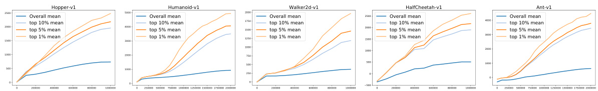
Figure 3: Training curves.
图 3: 训练曲线。
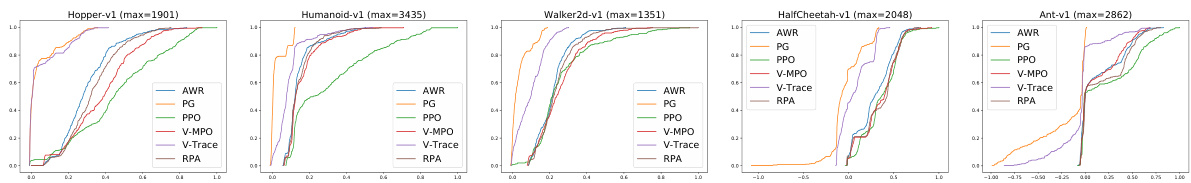
Figure 4: Empirical cumulative density functions of agent performance conditioned on different values of Policy loss (C14). The x axis denotes performance rescaled so that 0 corresponds to a random policy and 1 to the best found configuration, and the y axis denotes the quantile.
图 4: 基于不同策略损失 (C14) 值的智能体性能经验累积分布函数。x轴表示将性能重新缩放后的结果 (0对应随机策略,1对应最优配置),y轴表示分位数。
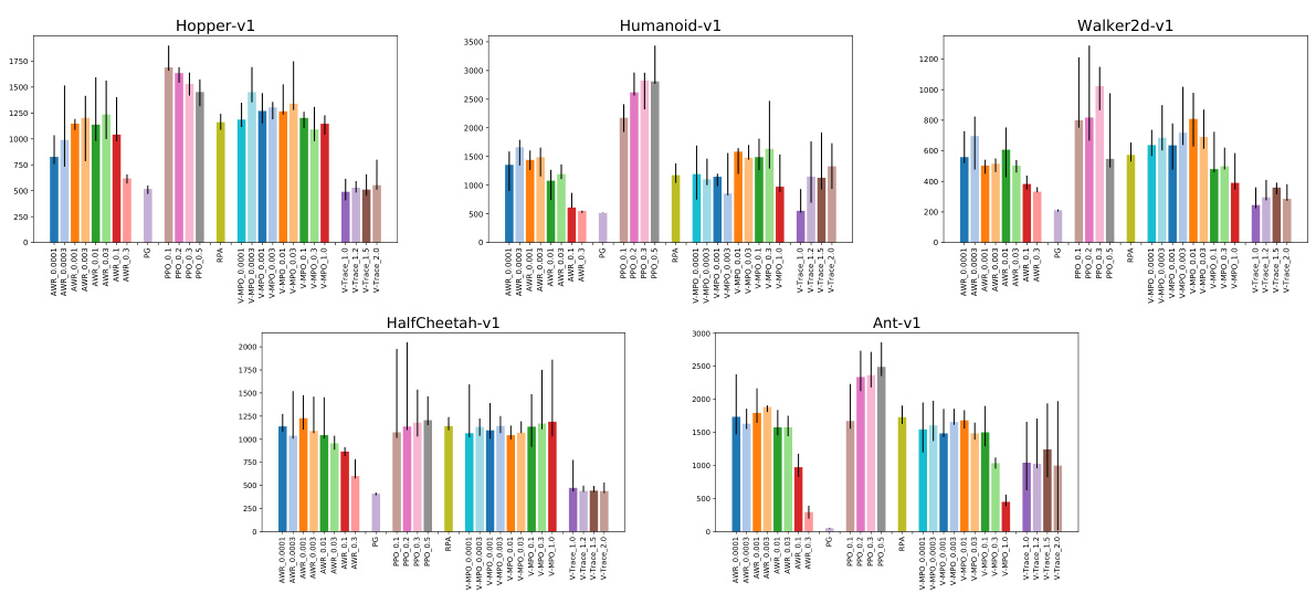
Figure 5: Comparison of 95th percentile of the performance of different policy losses conditioned on their hyper parameters.
图 5: 不同策略损失在超参数条件下的性能第95百分位对比。
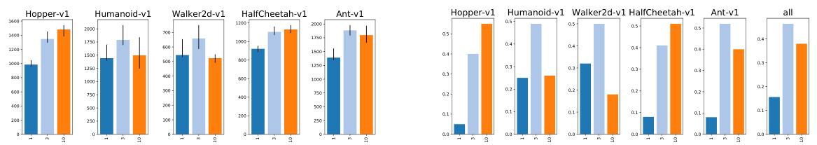
Figure 6: Analysis of choice num_epochs (C3): 95th percentile of performance scores conditioned on choice (left) and distribution of choices in top $5%$ of configurations (right).
图 6: 分析选择 num_epochs (C3):基于选择条件下的性能分数第95百分位(左)及前 $5%$ 配置中的选择分布(右)。
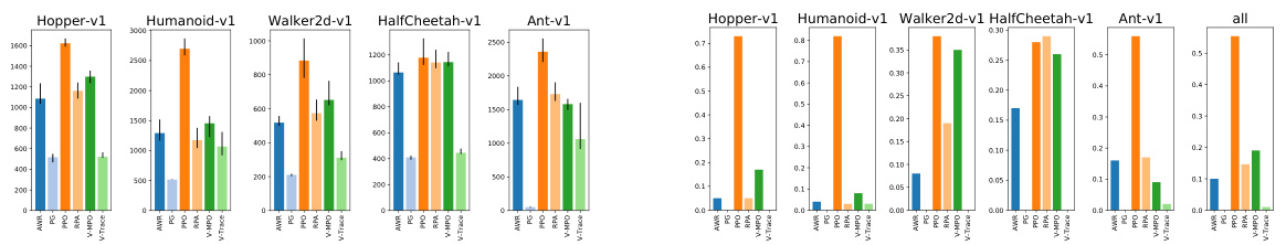
Figure 7: Analysis of choice Policy loss (C14): 95th percentile of performance scores conditioned on choice (left) and distribution of choices in top $5%$ of configurations (right).
图 7: 选择策略损失分析(C14): 基于选择条件的性能得分第95百分位(左)与最优 $5%$ 配置中的选择分布(右)。
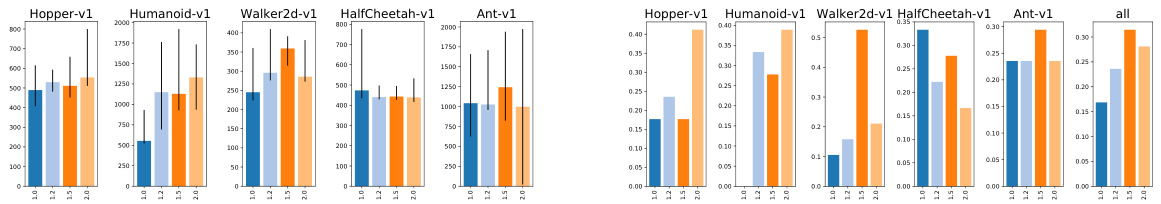
Figure 8: Analysis of choice V-Trace loss $\rho$ (C15): 95th percentile of performance scores conditioned on sub-choice (left) and distribution of sub-choices in top $5%$ of configurations (right).
图 8: 选择V-Trace损失 $\rho$ (C15)分析:基于子选择的性能得分第95百分位数(左)与配置前 $5%$ 中子选择分布(右)。
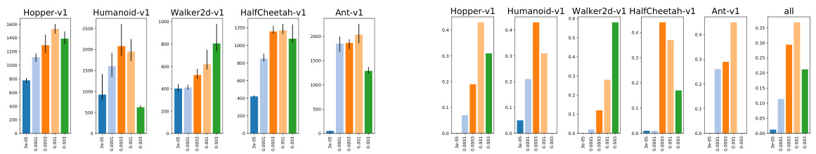
Figure 9: Analysis of choice Adam learning rate (C24): 95th percentile of performance scores conditioned on choice (left) and distribution of choices in top $5%$ of configurations (right).
图 9: 选择Adam学习率分析 (C24): 基于选择条件下的性能分数第95百分位 (左) 及前 $5%$ 配置中的选择分布 (右)。
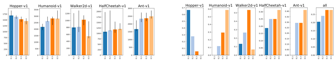
Figure 10: Analysis of choice PPO $\epsilon$ (C16): 95th percentile of performance scores conditioned on sub-choice (left) and distribution of sub-choices in top $5%$ of configurations (right).
图 10: 选择PPO $\epsilon$ 的分析(C16):基于子选择的性能分数第95百分位(左)与配置前 $5%$ 中子选择的分布(右)。
Figure 11: Analysis of choice V-MPO $\epsilon_{n}$ (C19): 95th percentile of performance scores conditioned on sub-choice (left) and distribution of sub-choices in top $5%$ of configurations (right).
图 11: 选择V-MPO的分析 $\epsilon_{n}$ (C19): 按子选择条件划分的性能分数第95百分位(左)及前 $5%$ 配置中子选择的分布(右)。
Figure 12: Analysis of choice AWR $\beta$ (C18): 95th percentile of performance scores conditioned on sub-choice (left) and distribution of sub-choices in top $5%$ of configurations (right).
图 12: 选择AWR $\beta$ (C18)的分析:基于子选择的性能分数第95百分位(左)及前$5%$配置中子选择的分布(右)。
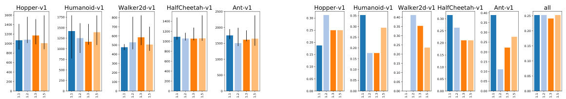
Figure 13: Analysis of choice AWR $\omega_{\mathtt{m a x}}$ (C17): 95th percentile of performance scores conditioned on sub-choice (left) and distribution of sub-choices in top $5%$ of configurations (right).
图 13: 选择AWR $\omega_{\mathtt{m a x}}$ (C17)的分析:基于子选择的性能分数95百分位(左)及前$5%$配置中子选择的分布(右)。

Figure 14: 95th percentile of performance scores conditioned on Policy loss (C14)(rows) and num_epochs (C3)(bars).
图 14: 基于策略损失(C14)(行)和训练轮数(C3)(柱)的性能分数第95百分位
E Experiment Networks architecture
E 实验网络架构
E.1 Design
E.1 设计
For each of the 5 environments, we sampled 4000 choice configurations where we sampled the following choices independently and uniformly from the following ranges:
对于这5种环境,我们分别采样了4000种选择配置,其中各项选择均从以下范围内独立且均匀地采样:
All the other choices were set to the default values as described in Appendix C.
其他所有选项均设置为附录C中所述的默认值。
For each of the sampled choice configurations, we train 3 agents with different random seeds and compute the performance metric as described in Section 2.
对于每个抽样的选择配置,我们使用不同的随机种子训练3个AI智能体,并按照第2节所述方法计算性能指标。
After running the experiment described above we noticed (Fig. 15) that separate policy and value function networks (C47) perform better and we have rerun the experiment with only this variant present.
运行上述实验后我们注意到(图15),独立的策略与价值函数网络(C47)表现更优,因此我们仅针对该变体重新进行了实验。
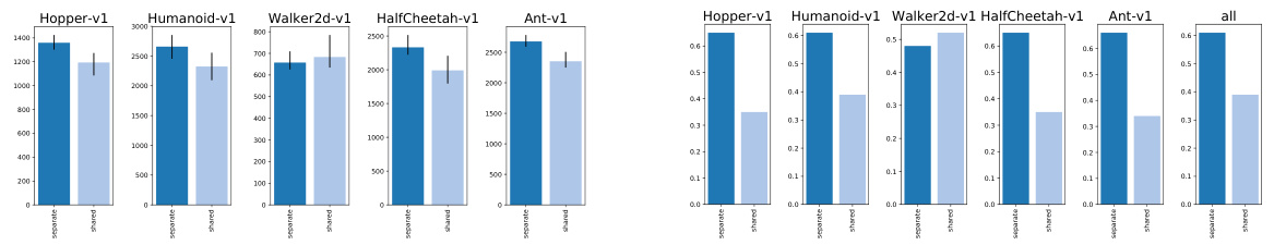
Figure 15: Analysis of choice Shared $\mathtt{M L P s}?$ (C47): 95th percentile of performance scores conditioned on choice (left) and distribution of choices in top $5%$ of configurations (right).
图 15: 共享 MLP 选择分析 (C47): 按选择条件筛选的性能得分第95百分位 (左) 及前5%配置中的选择分布 (右)。
E.2 Results
E.2 结果
We report aggregate statistics of the experiment in Table 4 as well as training curves in Figure 16. For each of the investigated choices in this experiment, we further provide a per-choice analysis in Figures 17-30.
我们在表4中报告了实验的汇总统计数据,并在图16中展示了训练曲线。针对本实验中的每个研究选项,我们还在图17-30中进一步提供了逐项分析。
Table 4: Performance quantiles across choice configurations.
| Ant-v1 | HalfCheetah-v1 | Hopper-v1 | Humanoid-v1 | Walker2d-v1 | |
| 90th percentile | 2098 | 1513 | 1133 | 1817 | 528 |
| 95th percentile | 2494 | 2120 | 1349 | 2382 | 637 |
| 99th percentile | 3138 | 3031 | 1582 | 3202 | 934 |
| Max | 4112 | 4358 | 1875 | 3987 | 1265 |
表 4: 不同选择配置下的性能分位数。
| Ant-v1 | HalfCheetah-v1 | Hopper-v1 | Humanoid-v1 | Walker2d-v1 | |
|---|---|---|---|---|---|
| 90th percentile | 2098 | 1513 | 1133 | 1817 | 528 |
| 95th percentile | 2494 | 2120 | 1349 | 2382 | 637 |
| 99th percentile | 3138 | 3031 | 1582 | 3202 | 934 |
| Max | 4112 | 4358 | 1875 | 3987 | 1265 |

Figure 16: Training curves.
图 16: 训练曲线。

Figure 17: Analysis of choice Action transformation $T_{u}$ (C63): 95th percentile of performance scores conditioned on choice (left) and distribution of choices in top $5%$ of configurations (right).
图 17: 选择动作变换 $T_{u}$ (C63) 分析:基于选择条件的性能得分第95百分位(左)及前 $5%$ 配置中的选择分布(右)。

Figure 18: Analysis of choice Policy MLP width (C49): 95th percentile of performance scores conditioned on choice (left) and distribution of choices in top $5%$ of configurations (right).
图 18: 选择策略MLP宽度分析(C49): 基于选择条件的性能分数第95百分位(左)与Top $5%$ 配置中的选择分布(右)。

Figure 19: Analysis of choice Last value layer scaling (C58): 95th percentile of performance scores conditioned on choice (left) and distribution of choices in top $5%$ of configurations (right).
图 19: 选择末值层缩放 (C58) 分析:基于选择的性能分数第95百分位 (左) 和配置前 $5%$ 的选择分布 (右)。

Figure 20: Analysis of choice Value MLP depth (C53): 95th percentile of performance scores conditioned on choice (left) and distribution of choices in top $5%$ of configurations (right).
图 20: 选择值 MLP (多层感知机) 深度分析 (C53): 基于选择的性能得分第95百分位 (左) 及前 $5%$ 配置中的选择分布 (右)。

Figure 21: Analysis of choice Value MLP width (C50): 95th percentile of performance scores conditioned on choice (left) and distribution of choices in top $5%$ of configurations (right).
图 21: 选择值MLP宽度分析(C50): 基于选择条件的性能分数第95百分位(左)及前$5%$配置中的选择分布(右)。

Figure 22: Analysis of choice Policy MLP depth (C52): 95th percentile of performance scores conditioned on choice (left) and distribution of choices in top $5%$ of configurations (right).
图 22: 选择策略MLP深度分析(C52): 按选择条件排序的性能分数第95百分位(左)及前$5%$配置中的选择分布(右)。

Figure 23: Analysis of choice Global standard deviation? (C59): 95th percentile of performance scores conditioned on choice (left) and distribution of choices in top $5%$ of configurations (right).
图 23: 选择全局标准差分析?(C59): 基于选择的性能分数第95百分位(左)与顶部$5%$配置中的选择分布(右)。

Figure 24: Analysis of choice Last policy layer scaling (C57): 95th percentile of performance scores conditioned on choice (left) and distribution of choices in top $5%$ of configurations (right).
图 24: 选择策略最后一层缩放分析 (C57):基于选择的性能分数第95百分位(左)及前 $5%$ 配置中的选择分布(右)。

Figure 25: Analysis of choice Standard deviation transformation $T_{\rho}$ (C60): 95th percentile of performance scores conditioned on choice (left) and distribution of choices in top $5%$ of configurations (right).
图 25: 选择标准差变换 $T_{\rho}$ (C60) 分析:基于选择的性能分数第95百分位 (左) 及前 $5%$ 配置中的选择分布 (右)。

Figure 26: Analysis of choice Adam learning rate (C24): 95th percentile of performance scores conditioned on choice (left) and distribution of choices in top $5%$ of configurations (right).
图 26: Adam学习率选择分析(C24):基于选择的性能得分95百分位(左)与最优 $5%$ 配置中的选择分布(右)。

Figure 27: Analysis of choice Initialize r (C56): 95th percentile of performance scores conditioned on choice (left) and distribution of choices in top $5%$ of configurations (right).
图 27: 选择初始化 r (C56) 的分析:基于选择条件的性能得分第95百分位 (左) 和配置前 $5%$ 的选择分布 (右)。

Figure 28: Analysis of choice Initial standard deviation $i_{\rho}$ (C61): 95th percentile of performance scores conditioned on choice (left) and distribution of choices in top $5%$ of configurations (right).
图 28: 初始标准差选择分析 $i_{\rho}$ (C61): 基于选择的性能分数第95百分位(左)与配置前 $5%$ 中的选择分布(右)。

Figure 29: Analysis of choice Minimum standard deviation $\epsilon_{\rho}$ (C62): 95th percentile of performance scores conditioned on choice (left) and distribution of choices in top $5%$ of configurations (right).
图 29: 选择最小标准差分析 $\epsilon_{\rho}$ (C62): 基于选择的性能分数第95百分位(左)及前 $5%$ 配置中的选择分布(右)。

Figure 30: Analysis of choice Activation (C55): 95th percentile of performance scores conditioned on choice (left) and distribution of choices in top $5%$ of configurations (right).
图 30: 选择激活(C55)分析:基于选择条件的性能分数第95百分位(左)与最优 $5%$ 配置中的选择分布(右)。
F Experiment Normalization and clipping
F 实验归一化与截断处理
F.1 Design
F.1 设计
For each of the 5 environments, we sampled 2000 choice configurations where we sampled the following choices independently and uniformly from the following ranges:
对于这5种环境中的每一种,我们采样了2000个选择配置,其中以下选择从以下范围内独立且均匀地采样:
All the other choices were set to the default values as described in Appendix C.
其他所有选项均设置为附录C中所述的默认值。
For each of the sampled choice configurations, we train 3 agents with different random seeds and compute the performance metric as described in Section 2.
对于每个抽样的选择配置,我们使用不同的随机种子训练3个AI智能体,并按照第2节所述计算性能指标。
F.2 Results
F.2 结果
We report aggregate statistics of the experiment in Table 5 as well as training curves in Figure 31. For each of the investigated choices in this experiment, we further provide a per-choice analysis in Figures 32-38.
我们在表5中报告了实验的汇总统计数据,并在图31中展示了训练曲线。对于本实验中的每个研究选项,我们还在图32-38中进一步提供了逐项分析。
Table 5: Performance quantiles across choice configurations.
| Ant-v1 | HalfCheetah-v1 | Hopper-vl | Humanoid-v1 | Walker2d-v1 | |
| 90th percentile | 2058 | 1265 | 1533 | 1649 | 1143 |
| 95th percentile | 2287 | 1716 | 1662 | 2165 | 1564 |
| 99th percentile | 2662 | 2465 | 1809 | 3100 | 2031 |
| Max | 3333 | 3515 | 2074 | 3482 | 2371 |
表 5: 不同选择配置下的性能分位数
| Ant-v1 | HalfCheetah-v1 | Hopper-vl | Humanoid-v1 | Walker2d-v1 | |
|---|---|---|---|---|---|
| 90th percentile | 2058 | 1265 | 1533 | 1649 | 1143 |
| 95th percentile | 2287 | 1716 | 1662 | 2165 | 1564 |
| 99th percentile | 2662 | 2465 | 1809 | 3100 | 2031 |
| Max | 3333 | 3515 | 2074 | 3482 | 2371 |

Figure 31: Training curves.
图 31: 训练曲线。

Figure 32: Analysis of choice PPO $\epsilon$ (C16): 95th percentile of performance scores conditioned on choice (left) and distribution of choices in top $5%$ of configurations (right).
图 32: 选择 PPO $\epsilon$ 的分析 (C16): 按选择条件划分的性能分数第95百分位 (左) 和配置前 $5%$ 中的选择分布 (右)。

Figure 33: Analysis of choice Input normalization (C64): 95th percentile of performance scores conditioned on choice (left) and distribution of choices in top $5%$ of configurations (right).
图 33: 选择输入归一化分析 (C64): 按选择条件划分的性能分数第95百分位 (左) 及前 $5%$ 配置中的选择分布 (右)。

Figure 34: Analysis of choice Gradient clipping (C68): 95th percentile of performance scores conditioned on choice (left) and distribution of choices in top $5%$ of configurations (right).
图 34: 选择梯度裁剪 (C68) 分析:基于选择条件的性能分数第95百分位 (左) 及前 $5%$ 配置中的选择分布 (右)。

Figure 35: Analysis of choice Per minibatch advantage normalization (C67): 95th percentile of performance scores conditioned on choice (left) and distribution of choices in top $5%$ of configurations (right).
图 35: 小批量优势归一化选择分析 (C67): 按选择分组的性能分数第95百分位 (左) 及前 $5%$ 配置中的选择分布 (右)。

Figure 36: Analysis of choice Adam learning rate (C24): 95th percentile of performance scores conditioned on choice (left) and distribution of choices in top $5%$ of configurations (right).
图 36: Adam学习率选择分析(C24): 基于选择条件下的性能分数第95百分位(左)与最优 $5%$ 配置中的选择分布(右)。

Figure 37: Analysis of choice Value function normalization (C66): 95th percentile of performance scores conditioned on choice (left) and distribution of choices in top $5%$ of configurations (right).
图 37: 选择价值函数归一化分析 (C66): 按选择条件划分的性能分数第95百分位 (左) 及前 $5%$ 配置中的选择分布 (右)。

Figure 38: Analysis of choice Input clipping (C65): 95th percentile of performance scores conditioned on sub-choice (left) and distribution of sub-choices in top $5%$ of configurations (right).
图 38: 选择输入截断分析 (C65): 按子选择分组的性能得分第95百分位数(左)及最优 $5%$ 配置中子选择的分布(右)。
G Experiment Advantage Estimation
G 实验优势估计
G.1 Design
G.1 设计
For each of the 5 environments, we sampled 4000 choice configurations where we sampled the following choices independently and uniformly from the following ranges:
对于每个环境,我们采样了4000种选择配置,其中各项选择均独立且均匀地从以下范围中采样:
All the other choices were set to the default values as described in Appendix C.
其他选项均按照附录C中的描述设为默认值。
For each of the sampled choice configurations, we train 3 agents with different random seeds and compute the performance metric as described in Section 2.
对于每个采样的选择配置,我们使用不同的随机种子训练3个AI智能体,并按照第2节所述计算性能指标。
G.2 Results
G.2 结果
We report aggregate statistics of the experiment in Table 6 as well as training curves in Figure 39. For each of the investigated choices in this experiment, we further provide a per-choice analysis in Figures 40-50.
我们在表6中报告了实验的汇总统计数据,并在图39中展示了训练曲线。对于本实验中的每个研究选项,我们还在图40-50中进一步提供了逐项分析。
Table 6: Performance quantiles across choice configurations.
| Ant-v1 | HalfCheetah-v1 | Hopper-vl | Humanoid-v1 | Walker2d-v1 | |
| 90th percentile | 1705 | 1128 | 1626 | 1922 | 947 |
| 95th percentile | 2114 | 1535 | 1777 | 2374 | 1185 |
| 99th percentile | 2781 | 2631 | 2001 | 3013 | 1697 |
| Max | 3775 | 3613 | 2215 | 3564 | 2309 |
表 6: 不同选择配置下的性能分位数
| Ant-v1 | HalfCheetah-v1 | Hopper-vl | Humanoid-v1 | Walker2d-v1 | |
|---|---|---|---|---|---|
| 90th percentile | 1705 | 1128 | 1626 | 1922 | 947 |
| 95th percentile | 2114 | 1535 | 1777 | 2374 | 1185 |
| 99th percentile | 2781 | 2631 | 2001 | 3013 | 1697 |
| Max | 3775 | 3613 | 2215 | 3564 | 2309 |

Figure 39: Training curves.
图 39: 训练曲线。

Figure 40: Comparison of 95th percentile of the performance of different advantage estimators conditioned on their hyper parameters.
图 40: 不同优势估计器在超参数条件下的第95百分位性能对比

Figure 41: Analysis of choice num_envs (C1): 95th percentile of performance scores conditioned on choice (left) and distribution of choices in top $5%$ of configurations (right).
图 41: 环境数量选择分析 (C1):基于选择条件的性能得分第95百分位(左)及前 $5%$ 配置中的选择分布(右)。

Figure 42: Analysis of choice Value function loss (C11): 95th percentile of performance scores conditioned on choice (left) and distribution of choices in top $5%$ of configurations (right).
图 42: 选择值函数损失分析 (C11): 基于选择的性能得分第95百分位数 (左) 和配置前 $5%$ 中的选择分布 (右)。

Figure 43: Analysis of choice PPO-style value clipping $\epsilon$ (C13): 95th percentile of performance scores conditioned on choice (left) and distribution of choices in top $5%$ of configurations (right).
图 43: PPO式价值剪裁参数 $\epsilon$ (C13)的选择分析:基于选择条件下的性能得分第95百分位(左)及前 $5%$ 配置中的选择分布(右)。

Figure 44: Analysis of choice advantage estimator (C6): 95th percentile of performance scores conditioned on choice (left) and distribution of choices in top $5%$ of configurations (right).
图 44: 选择优势估计器 (C6) 分析:基于选择条件下的性能分数第95百分位 (左) 及前 $5%$ 配置中的选择分布 (右)。

Figure 45: Analysis of choice GAE $\lambda$ (C8): 95th percentile of performance scores conditioned on sub-choice (left) and distribution of sub-choices in top $5%$ of configurations (right).
图 45: 选择GAE $\lambda$ 的分析(C8): 基于子选择的性能分数第95百分位数(左)及前$5%$配置中子选择的分布(右)。

Figure 46: Analysis of choice Adam learning rate (C24): 95th percentile of performance scores conditioned on choice (left) and distribution of choices in top $5%$ of configurations (right).
图 46: 选择 Adam 学习率 (C24) 的分析:基于选择的性能分数第 95 百分位 (左) 和配置前 $5%$ 中的选择分布 (右)。

Figure 47: Analysis of choice N-step $N$ (C7): 95th percentile of performance scores conditioned on sub-choice (left) and distribution of sub-choices in top $5%$ of configurations (right).
图 47: 选择N步长 $N$ (C7)分析:基于子选项的性能分数第95百分位(左)及前 $5%$ 配置中子选项的分布(右)。

Figure 48: Analysis of choice Huber delta (C12): 95th percentile of performance scores conditioned on sub-choice (left) and distribution of sub-choices in top $5%$ of configurations (right).
图 48: 选择 Huber delta (C12) 分析:基于子选项的性能分数第95百分位数 (左) 和配置前 $5%$ 中子选项的分布 (右)。

Figure 49: Analysis of choice V-Trace advantage $\lambda$ (C9): 95th percentile of performance scores conditioned on sub-choice (left) and distribution of sub-choices in top $5%$ of configurations (right).
图 49: V-Trace优势参数 $\lambda$ 选择分析 (C9): 子选项条件下性能得分的95百分位 (左) 及前 $5%$ 配置中子选项的分布 (右)。

Figure 50: Analysis of choice V-Trace advantage c, $\rho$ (C10): 95th percentile of performance scores conditioned on sub-choice (left) and distribution of sub-choices in top $5%$ of configurations (right).
图 50: 选择V-Trace优势c的分析,$\rho$ (C10):基于子选择的性能分数第95百分位数(左)及前$5%$配置中子选择的分布(右)。
H Experiment Training setup
H 实验训练设置
H.1 Design
H.1 设计
For each of the 5 environments, we sampled 2000 choice configurations where we sampled the following choices independently and uniformly from the following ranges:
对于5种环境中的每一种,我们采样了2000种选择配置,其中以下选项均从给定范围内独立且均匀采样:
All the other choices were set to the default values as described in Appendix C.
其他所有选项均设置为附录C中所述的默认值。
For each of the sampled choice configurations, we train 3 agents with different random seeds and compute the performance metric as described in Section 2.
对于每个采样的选择配置,我们使用不同的随机种子训练3个AI智能体,并按照第2节所述计算性能指标。
H.2 Results
H.2 结果
We report aggregate statistics of the experiment in Table 7 as well as training curves in Figure 51. For each of the investigated choices in this experiment, we further provide a per-choice analysis in Figures 52-58.
我们在表7中报告了实验的汇总统计数据,并在图51中展示了训练曲线。对于本实验中的每个研究选项,我们还在图52-58中进一步提供了逐项分析。
Table 7: Performance quantiles across choice configurations.
| Ant-v1 | HalfCheetah-v1 | Hopper-v1 | Humanoid-v1 | Walker2d-v1 | |
| 90th percentile | 2203 | 1316 | 1695 | 2310 | 1190 |
| 95th percentile | 2484 | 1673 | 1853 | 2655 | 1431 |
| 99th percentile | 2907 | 2665 | 2060 | 3014 | 1844 |
| Max | 3563 | 3693 | 2434 | 3502 | 2426 |
表 7: 不同选择配置下的性能分位数。
| Ant-v1 | HalfCheetah-v1 | Hopper-v1 | Humanoid-v1 | Walker2d-v1 | |
|---|---|---|---|---|---|
| 90分位数 | 2203 | 1316 | 1695 | 2310 | 1190 |
| 95分位数 | 2484 | 1673 | 1853 | 2655 | 1431 |
| 99分位数 | 2907 | 2665 | 2060 | 3014 | 1844 |
| 最大值 | 3563 | 3693 | 2434 | 3502 | 2426 |

Figure 51: Training curves.
图 51: 训练曲线。

Figure 52: Analysis of choice iteration size (C2): 95th percentile of performance scores conditioned on choice (left) and distribution of choices in top $5%$ of configurations (right).
图 52: 选择迭代大小分析(C2):基于选择的性能得分第95百分位数(左)与最优配置前$5%$中的选择分布(右)。

Figure 53: Analysis of choice batch_mode (C5): 95th percentile of performance scores conditioned on choice (left) and distribution of choices in top $5%$ of configurations (right).
图 53: 选择批次模式 (C5) 分析:基于选择的性能分数第95百分位 (左) 及前 $5%$ 配置中的选择分布 (右)。

Figure 54: Analysis of choice num_epochs (C3): 95th percentile of performance scores conditioned on choice (left) and distribution of choices in top $5%$ of configurations (right).
图 54: num_epochs选择分析(C3):基于选择条件的性能分数第95百分位(左)与配置前$5%$中的选择分布(右)。

Figure 55: Analysis of choice num_envs (C1): 95th percentile of performance scores conditioned on choice (left) and distribution of choices in top $5%$ of configurations (right).
图 55: 选择 num_envs (C1) 的分析:基于选择条件下的性能分数第95百分位 (左) 和配置前 $5%$ 中的选择分布 (右)。

Figure 56: Analysis of choice Adam learning rate (C24): 95th percentile of performance scores conditioned on choice (left) and distribution of choices in top $5%$ of configurations (right).
图 56: Adam学习率选择分析(C24): 基于选择的性能分数95百分位值(左)与配置前$5%$的选择分布(右)。

Figure 57: Analysis of choice batch_size (C4): 95th percentile of performance scores conditioned on choice (left) and distribution of choices in top $5%$ of configurations (right).
图 57: 批次大小选择分析(C4):基于选择条件的性能分数第95百分位(左)与最优 $5%$ 配置中的选择分布(右)。

Figure 58: Analysis of choice batch_mode (C5): 95th percentile of performance scores conditioned on choice (left) and distribution of choices in top $5%$ of configurations(right). In order to obtain narrower confidence intervals in this experiment we only sweep batch_mode (C5), num_envs (C1), Adam learning rate (C24).
图 58: 选择batch_mode (C5)的分析:基于选择的性能分数第95百分位(左)与配置前$5%$中的选择分布(右)。为在本实验中获得更窄的置信区间,我们仅扫描batch_mode (C5)、num_envs (C1)和Adam学习率(C24)。
I Experiment Time
I 实验时间
I.1 Design
I.1 设计
For each of the 5 environments, we sampled 2000 choice configurations where we sampled the following choices independently and uniformly from the following ranges:
对于这5种环境,我们分别采样了2000种选择配置,其中各项选择均从以下范围内独立且均匀地采样:
Discount factor $\gamma$ (C20): {0.95, 0.97, 0.99, 0.999} Frame skip (C21): {1, 2, 5} • Handle abandoned? (C22): {False, True} Adam learning rate (C24): {3e-05, 0.0001, 0.0003, 0.001}
折扣因子 $\gamma$ (C20): {0.95, 0.97, 0.99, 0.999}
帧跳过 (C21): {1, 2, 5}
• 处理弃用状态? (C22): {False, True}
Adam学习率 (C24): {3e-05, 0.0001, 0.0003, 0.001}
All the other choices were set to the default values as described in Appendix C.
其他所有选项均设置为附录C中所述的默认值。
For each of the sampled choice configurations, we train 3 agents with different random seeds and compute the performance metric as described in Section 2.
对于每个抽样的选择配置,我们使用不同的随机种子训练3个AI智能体,并按照第2节所述计算性能指标。
I.2 Results
I.2 结果
We report aggregate statistics of the experiment in Table 8 as well as training curves in Figure 59. For each of the investigated choices in this experiment, we further provide a per-choice analysis in Figures 60-63.
我们在表8中报告了实验的汇总统计数据,并在图59中展示了训练曲线。针对本实验中的每个研究选项,我们在图60-63中进一步提供了逐项分析。
Table 8: Performance quantiles across choice configurations
| Ant-v1 | HalfCheetah-v1 | Hopper-v1 | Humanoid-v1 | Walker2d-v1 | |
| 90th percentile | 1462 | 1063 | 1243 | 1431 | 761 |
| 95th percentile | 1654 | 1235 | 1675 | 2158 | 810 |
| 99th percentile | 2220 | 1423 | 2204 | 2769 | 974 |
| Max | 2833 | 1918 | 2434 | 3106 | 1431 |
表 8: 不同选择配置下的性能分位数
| Ant-v1 | HalfCheetah-v1 | Hopper-v1 | Humanoid-v1 | Walker2d-v1 | |
|---|---|---|---|---|---|
| 90th percentile | 1462 | 1063 | 1243 | 1431 | 761 |
| 95th percentile | 1654 | 1235 | 1675 | 2158 | 810 |
| 99th percentile | 2220 | 1423 | 2204 | 2769 | 974 |
| Max | 2833 | 1918 | 2434 | 3106 | 1431 |

Figure 59: Training curves.
图 59: 训练曲线。

Figure 60: Analysis of choice Discount factor $\gamma$ (C20): 95th percentile of performance scores conditioned on choice (left) and distribution of choices in top $5%$ of configurations (right).
图 60: 选择折扣因子 $\gamma$ (C20) 分析:基于选择的性能得分第95百分位 (左) 及前 $5%$ 配置中的选择分布 (右)。

Figure 61: Analysis of choice Frame skip (C21): 95th percentile of performance scores conditioned on choice (left) and distribution of choices in top $5%$ of configurations (right).
图 61: 选择帧跳过 (C21) 分析:基于选择的性能分数第95百分位(左)及前 $5%$ 配置中的选择分布(右)。

Figure 62: Analysis of choice Handle abandoned? (C22): 95th percentile of performance scores conditioned on choice (left) and distribution of choices in top $5%$ of configurations (right).
图 62: 选项处理放弃情况分析 (C22): 基于选项的性能分数第95百分位值 (左) 和最优 $5%$ 配置中的选项分布 (右)。

Figure 63: Analysis of choice Adam learning rate (C24): 95th percentile of performance scores conditioned on choice (left) and distribution of choices in top $5%$ of configurations (right).
图 63: Adam学习率选择分析(C24): 按选择条件划分的性能分数第95百分位(左)及前$5%$配置中的选择分布(右)。
J Experiment Optimizers
J 实验优化器
J.1 Design
J.1 设计
For each of the 5 environments, we sampled 2000 choice configurations where we sampled the following choices independently and uniformly from the following ranges:
对于每个环境,我们独立均匀采样了2000种选择配置,采样范围如下:
All the other choices were set to the default values as described in Appendix C.
其他所有选项均设置为附录C中所述的默认值。
For each of the sampled choice configurations, we train 3 agents with different random seeds and compute the performance metric as described in Section 2.
对于每个抽样的选择配置,我们用不同的随机种子训练3个AI智能体,并按照第2节所述计算性能指标。
J.2 Results
J.2 结果
We report aggregate statistics of the experiment in Table 9 as well as training curves in Figure 64. For each of the investigated choices in this experiment, we further provide a per-choice analysis in Figures 65-73.
我们在表9中报告了实验的汇总统计数据,并在图64中展示了训练曲线。对于本实验中的每个研究选项,我们还在图65-73中进一步提供了逐项分析。
Table 9: Performance quantiles across choice configurations.
| Ant-v1 | HalfCheetah-v1 | Hopper-v1 | Humanoid-v1 | Walker2d-v1 | |
| 90th percentile | 2180 | 1085 | 1675 | 2549 | 712 |
| 95th percentile | 2388 | 1124 | 1728 | 2726 | 797 |
| 99th percentile | 2699 | 1520 | 1826 | 2976 | 1079 |
| Max | 2953 | 2532 | 1959 | 3332 | 1453 |
表 9: 不同选择配置下的性能分位数
| Ant-v1 | HalfCheetah-v1 | Hopper-v1 | Humanoid-v1 | Walker2d-v1 | |
|---|---|---|---|---|---|
| 90th percentile | 2180 | 1085 | 1675 | 2549 | 712 |
| 95th percentile | 2388 | 1124 | 1728 | 2726 | 797 |
| 99th percentile | 2699 | 1520 | 1826 | 2976 | 1079 |
| Max | 2953 | 2532 | 1959 | 3332 | 1453 |

Figure 64: Training curves.
图 64: 训练曲线。

Figure 65: Analysis of choice Learning rate decay (C31): 95th percentile of performance scores conditioned on choice (left) and distribution of choices in top $5%$ of configurations (right).
图 65: 学习率衰减选择分析 (C31): 按选择条件划分的性能分数第95百分位 (左) 及前 $5%$ 配置中的选择分布 (右)。

Figure 66: Analysis of choice Optimizer (C23): 95th percentile of performance scores conditioned on choice (left) and distribution of choices in top $5%$ of configurations (right).
图 66: 选择优化器 (C23) 分析:基于选择条件的性能分数第95百分位 (左) 和配置前 $5%$ 中的选择分布 (右)。

Figure 67: Analysis of choice Adam momentum (C26): 95th percentile of performance scores conditioned on sub-choice (left) and distribution of sub-choices in top $5%$ of configurations (right).
图 67: 选择Adam动量(C26)的分析:基于子选择条件下的性能得分第95百分位(左)与配置前$5%$中子选择的分布(右)。

Figure 68: Analysis of choice Adam $\epsilon$ (C28): 95th percentile of performance scores conditioned on sub-choice (left) and distribution of sub-choices in top $5%$ of configurations (right).
图 68: Adam优化器 $\epsilon$ 参数选择分析 (C28): 按子选项分组的性能得分第95百分位 (左) 及前 $5%$ 配置中子选项的分布情况 (右)。

Figure 69: Analysis of choice Adam learning rate (C24): 95th percentile of performance scores conditioned on sub-choice (left) and distribution of sub-choices in top $5%$ of configurations (right).
图 69: Adam学习率选择分析(C24):基于子选项的性能分数第95百分位(左)与最优 $5%$ 配置中子选项的分布(右)。

Figure 70: Analysis of choice RMSProp centered? (C30): 95th percentile of performance scores conditioned on sub-choice (left) and distribution of sub-choices in top $5%$ of configurations (right).
图 70: 中心化选项RMSProp分析? (C30): 基于子选项的性能分数第95百分位(左)与配置前$5%$中子选项的分布(右)。

Figure 71: Analysis of choice RMSProp momentum (C27): 95th percentile of performance scores conditioned on sub-choice (left) and distribution of sub-choices in top $5%$ of configurations (right).
图 71: 选择RMSProp动量(C27)分析:基于子选择的性能得分第95百分位(左)及前$5%$配置中子选择的分布(右)。

Figure 72: Analysis of choice RMSProp ϵ (C29): 95th percentile of performance scores conditioned on sub-choice (left) and distribution of sub-choices in top $5%$ of configurations (right).
图 72: 选择 RMSProp ϵ (C29) 的分析:基于子选择的性能分数第 95 百分位数 (左) 和 top $5%$ 配置中子选择的分布 (右)。

Figure 73: Analysis of choice RMSProp learning rate (C25): 95th percentile of performance scores conditioned on sub-choice (left) and distribution of sub-choices in top $5%$ of configurations (right).
图 73: RMSProp学习率选择分析(C25): 子选项条件下性能得分的95百分位(左)及前 $5%$ 配置中子选项的分布(右)。

Figure 74: 95th percentile of performance scores conditioned on RMSProp momentum (C27)(rows) and RMSProp learning rate (C25)(bars).
图 74: 基于 RMSProp 动量 (C27)(行) 和 RMSProp 学习率 (C25)(柱) 的性能分数第95百分位。
K Experiment Regularize rs
K 实验正则化器
K.1 Design
K.1 设计
For each of the 5 environments, we sampled 4000 choice configurations where we sampled the following choices independently and uniformly from the following ranges:
对于每个环境,我们采样了4000种选择配置,其中各项选择均从以下范围内独立且均匀地采样:

- 正则化类型 (C32): {约束, 无正则化, 惩罚}
- 当"正则化类型 (C32) = 约束"时,进一步采样子选项:
* 约束型正则化器 (C34): {KL(μ||π), KL(π||μ), KL(ref||π), 解耦KL(μ||π), 熵}
$\diamond$ 当"约束型正则化器 (C34)=KL(μ||π)"时,进一步采样子选项:
– KL(μ||π)阈值 (C35): {0.005, 0.01, 0.02, 0.04, 0.08}
$\diamond$ 当"约束型正则化器 (C34)=KL(π||μ)"时,进一步采样子选项:
– KL(π||μ)阈值 (C36): {0.005, 0.01, 0.02, 0.04, 0.08}
$\diamond$ 当"约束型正则化器 (C34)=KL(ref||π)"时,进一步采样子选项:
– KL(ref||π)阈值 (C37): {10.0, 20.0, 40.0, 80.0, 160.0}
$\diamond$ 当"约束型正则化器 (C34)=解耦KL(μ||π)"时,进一步采样子选项:
– 解耦KL均值阈值 (μ||π) (C38): {0.005, 0.01, 0.02, 0.04, 0.08}
– 解耦KL标准差阈值 (μ||π) (C39): {5e-05, 0.000125, 0.00025, 0.0005, 0.001, 0.002, 0.004}
$\diamond$ 当"约束型正则化器 (C34)=熵"时,进一步采样子选项:
– 熵阈值 H(π) (C40): {0.0, -5.0, -10.0, -15.0} - 当"正则化类型 (C32) = 惩罚"时,进一步采样子选项:
* 惩罚型正则化器 (C33): {KL(μ||π), KL(π||μ), KL(ref||π), 解耦KL(μ||π), 熵}
$\diamond$ 当"惩罚型正则化器 (C33)=KL(μ||π)"时,进一步采样子选项:
– KL(μ||π)系数 (C41): {0.003, 0.01, 0.03, 0.1, 0.3, 1.0}
$\diamond$ 当"惩罚型正则化器 (C33)=KL(π||μ)"时,进一步采样子选项:
– KL(π||μ)系数 (C42): {0.003, 0.01, 0.03, 0.1, 0.3, 1.0}
$\diamond$ 当"惩罚型正则化器 (C33)=KL(ref||π)"时,进一步采样子选项:
– KL(ref||π)系数 (C43): {3e-06, 1e-05, 3e-05, 0.0001, 0.0003, 0.001}
$\diamond$ 当"惩罚型正则化器 (C33)=解耦KL(μ||π)"时,进一步采样子选项:
– 解耦KL均值系数 (μ||π) (C44): {0.003, 0.01, 0.03, 0.1, 0.3, 1.0}
– 解耦KL标准差系数 (μ||π) (C45): {0.1, 0.3, 1.0, 3.0, 10.0, 30.0, 100.0, 300.0}
$\diamond$ 当"惩罚型正则化器 (C33)=熵"时,进一步采样子选项:
– 熵系数 (C46): {1e-05, 3e-05, 0.0001, 0.0003, 0.001, 0.003}
- 当"正则化类型 (C32) = 约束"时,进一步采样子选项:
Adam学习率 (C24): {3e-05, 0.0001, 0.0003, 0.001, 0.003}
其他选项设置为附录C所述的默认值。对每个采样配置,我们使用3个不同随机种子训练智能体,并按第2节所述计算性能指标。
K.2 Results
K.2 结果
We report aggregate statistics of the experiment in Table 10 as well as training curves in Figure 75. For each of the investigated choices in this experiment, we further provide a per-choice analysis in Figures 76-92.
我们在表10中报告了实验的汇总统计结果,并在图75中展示了训练曲线。针对本实验中的每个研究选项,我们还在图76至图92中提供了逐项分析。
Table 10: Performance quantiles across choice configurations.
| Ant-v1 | HalfCheetah-v1 | Hopper-v1 | Humanoid-v1 | Walker2d-v1 | |
| 90th percentile | 2158 | 1477 | 1639 | 2624 | 705 |
| 95th percentile | 2600 | 1870 | 1707 | 2832 | 814 |
| 99th percentile | 2956 | 2413 | 1812 | 3071 | 1016 |
| Max | 3202 | 3156 | 1979 | 3348 | 1597 |
表 10: 不同选择配置下的性能分位数。
| Ant-v1 | HalfCheetah-v1 | Hopper-v1 | Humanoid-v1 | Walker2d-v1 | |
|---|---|---|---|---|---|
| 90th percentile | 2158 | 1477 | 1639 | 2624 | 705 |
| 95th percentile | 2600 | 1870 | 1707 | 2832 | 814 |
| 99th percentile | 2956 | 2413 | 1812 | 3071 | 1016 |
| Max | 3202 | 3156 | 1979 | 3348 | 1597 |

Figure 75: Training curves.
图 75: 训练曲线。

Figure 76: Comparison of 95th percentile of the performance of different regular iz ation approaches conditioned on their type.
图 76: 不同正则化方法在各自类型条件下性能的第95百分位对比

Figure 77: Analysis of choice Regular iz ation type (C32): 95th percentile of performance scores conditioned on choice (left) and distribution of choices in top $5%$ of configurations (right).
图 77: 正则化类型选择分析(C32):基于选择条件的性能得分第95百分位(左)与最优 $5%$ 配置中的选择分布(右)。

Figure 78: Analysis of choice Regularize r (in case of penalty) (C33): 95th percentile of performance scores conditioned on sub-choice (left) and distribution of sub-choices in top $5%$ of configurations (right).
图 78: 惩罚情形下正则化参数 r 的选择分析 (C33): 基于子选项的性能分数第95百分位数 (左) 及前 $5%$ 配置中子选项的分布情况 (右)。

Figure 79: Analysis of choice Regularize r coefficient for $\mathtt{K L}(\mathtt{r e f}||\pi)$ (C43): 95th percentile of performance scores conditioned on sub-choice (left) and distribution of sub-choices in top $5%$ of configurations (right).
图 79: 选择正则化系数 $\mathtt{K L}(\mathtt{r e f}||\pi)$ (C43) 的分析:基于子选择的性能分数第95百分位 (左) 和 top $5%$ 配置中子选择的分布 (右)。

Figure 80: Analysis of choice Adam learning rate (C24): 95th percentile of performance scores conditioned on choice (left) and distribution of choices in top $5%$ of configurations (right).
图 80: Adam学习率选择分析(C24):基于选择条件的性能分数第95百分位(左)及前$5%$配置中的选择分布(右)。

Figure 81: Analysis of choice Regularize r coefficient for entropy (C46): 95th percentile of performance scores conditioned on sub-choice (left) and distribution of sub-choices in top $5%$ of configurations (right).
图 81: 熵正则化系数 (C46) 选择分析:基于子选择的性能得分第95百分位数 (左) 及前 $5%$ 配置中子选择的分布 (右)。

Figure 82: Analysis of choice Regularize r (in case of constraint) (C34): 95th percentile of performance scores conditioned on sub-choice (left) and distribution of sub-choices in top $5%$ of configurations (right).
图 82: 约束条件下正则化参数 r 的选择分析 (C34) : 基于子选项的性能得分第95百分位数 (左) 及前 $5%$ 配置中子选项的分布情况 (右)。

Figure 83: Analysis of choice Threshold for entropy $H(\pi)$ (C40): 95th percentile of performance scores conditioned on sub-choice (left) and distribution of sub-choices in top $5%$ of configurations (right).
图 83: 熵选择阈值 $H(\pi)$ (C40) 分析:基于子选择的性能得分第95百分位数(左)与最优 $5%$ 配置中子选择的分布(右)。

Figure 84: Analysis of choice Threshold for $\mathtt{K L}(\mu||\pi)$ (C35): 95th percentile of performance scores conditioned on sub-choice (left) and distribution of sub-choices in top $5%$ of configurations (right).
图 84: 选择阈值 $\mathtt{K L}(\mu||\pi)$ (C35) 分析:基于子选择的性能得分第95百分位(左)与 top $5%$ 配置中子选择分布(右)。

Figure 85: Analysis of choice Regularize r coefficient for mean in decoupled $\mathtt{K L}(\mu||\pi)$ (C44): 95th percentile of performance scores conditioned on sub-choice (left) and distribution of sub-choices in top $5%$ of configurations (right).
图 85: 解耦 $\mathtt{K L}(\mu||\pi)$ 均值正则化系数选择分析 (C44): 基于子选项的性能分数第95百分位 (左) 及前 $5%$ 配置中子选项的分布 (右)。

Figure 86: Analysis of choice Regularize r coefficient for std in decoupled $\mathtt{K L}(\mu||\pi)$ (C45): 95th percentile of performance scores conditioned on sub-choice (left) and distribution of sub-choices in top $5%$ of configurations (right).
图 86: 解耦 $\mathtt{K L}(\mu||\pi)$ (C45) 中 std 的正则化系数选择分析:基于子选择的性能分数第95百分位 (左) 和 top $5%$ 配置中子选择的分布 (右)。

Figure 87: Analysis of choice Threshold for $\operatorname{KL}(\pi||\mu)$ (C36): 95th percentile of performance scores conditioned on sub-choice (left) and distribution of sub-choices in top $5%$ of configurations (right).
图 87: 选择阈值分析 $\operatorname{KL}(\pi||\mu)$ (C36):基于子选择的性能分数第95百分位(左)及前 $5%$ 配置中子选择的分布(右)。

Figure 88: Analysis of choice Regularize r coefficient for $\operatorname{KL}(\pi||\mu)$ (C42): 95th percentile of performance scores conditioned on sub-choice (left) and distribution of sub-choices in top $5%$ of configurations (right).
图 88: 选择正则化系数r对$\operatorname{KL}(\pi||\mu)$ (C42)的分析:基于子选择条件下的性能分数第95百分位数(左)及前$5%$配置中子选择的分布(右)。

Figure 89: Analysis of choice Threshold for mean in decoupled $\mathtt{K L}(\mu||\pi)$ (C38): 95th percentile of performance scores conditioned on sub-choice (left) and distribution of sub-choices in top $5%$ of configurations (right).
图 89: 解耦均值选择阈值分析 $\mathtt{K L}(\mu||\pi)$ (C38): 基于子选择的性能分数第95百分位(左)及前 $5%$ 配置中子选择分布(右)。

Figure 90: Analysis of choice Threshold for std in decoupled $\mathtt{K L}(\mu||\pi)$ (C39): 95th percentile of performance scores conditioned on sub-choice (left) and distribution of sub-choices in top $5%$ of configurations (right).
图 90: 解耦选择阈值分析 std 在 $\mathtt{K L}(\mu||\pi)$ (C39) 中的表现:基于子选择的性能分数第95百分位(左)及前 $5%$ 配置中子选择的分布(右)。

Figure 91: Analysis of choice Threshold for KL(ref $||\pi)$ (C37): 95th percentile of performance scores conditioned on sub-choice (left) and distribution of sub-choices in top $5%$ of configurations (right).
图 91: KL(ref $||\pi)$ 选择阈值分析 (C37) : 基于子选择条件的性能分数第95百分位 (左) 及前 $5%$ 配置中子选择的分布 (右) 。

Figure 92: Analysis of choice Regularize r coefficient for $\mathtt{K L}(\mu||\pi)$ (C41): 95th percentile of performance scores conditioned on sub-choice (left) and distribution of sub-choices in top $5%$ of configurations (right).
图 92: 针对 $\mathtt{K L}(\mu||\pi)$ (C41) 的正则化系数选择分析:基于子选择的性能得分第95百分位(左)及前 $5%$ 配置中子选择的分布(右)。