Tasks, stability, architecture, and compute: Training more effective learned optimizers, and using them to train themselves
任务、稳定性、架构与算力:训练更高效的学习型优化器及其自我训练应用
Luke Metz Google Research, Brain Team lmetz@google.com
Luke Metz Google Research, Brain Team lmetz@google.com
Niru Ma he s war a nathan Google Research, Brain Team nirum@google.com
Niru Maheswaranathan
Google Research, Brain Team
nirum@google.com
C. Daniel Freeman Google Research, Brain Team cdfreeman@google.com
C. Daniel Freeman Google Research, Brain Team cdfreeman@google.com
Ben Poole Google Research, Brain Team pooleb@google.com
Ben Poole Google Research, Brain Team pooleb@google.com
Jascha Sohl-Dickstein Google Research, Brain Team jaschasd@google.com
Jascha Sohl-Dickstein Google Research, Brain Team jaschasd@google.com
Abstract
摘要
Much as replacing hand-designed features with learned functions has revolutionized how we solve perceptual tasks, we believe learned algorithms will transform how we train models. In this work we focus on general-purpose learned optimizers capable of training a wide variety of problems with no user-specified hyperparameters. We introduce a new, neural network parameterized, hierarchical optimizer with access to additional features such as validation loss to enable automatic regularization. Most learned optimizers have been trained on only a single task, or a small number of tasks. We train our optimizers on thousands of tasks, making use of orders of magnitude more compute, resulting in optimizers that generalize better to unseen tasks. The learned optimizers not only perform well, but learn behaviors that are distinct from existing first order optimizers. For instance, they generate update steps that have implicit regular iz ation and adapt as the problem hyperparameters (e.g. batch size) or architecture (e.g. neural network width) change. Finally, these learned optimizers show evidence of being useful for out of distribution tasks such as training themselves from scratch.
正如通过学习函数替代手工设计的特征彻底改变了我们解决感知任务的方式一样,我们相信学习算法将重塑模型训练范式。本研究聚焦于无需用户指定超参数、能训练多种任务的通用学习型优化器。我们提出一种新型神经网络参数化的分层优化器,其可利用验证损失等附加特征实现自动正则化。现有学习型优化器大多仅在单一或少量任务上训练,而我们的优化器在数千个任务上训练,消耗了数量级更高的算力,从而获得更优秀的未知任务泛化能力。这些优化器不仅性能优异,还展现出与一阶优化器截然不同的行为特征:例如能生成具有隐式正则化的更新步骤,并随问题超参数(如批量大小)或架构(如神经网络宽度)变化而自适应调整。最后,这些学习型优化器还显示出对分布外任务(如从零开始自我训练)的潜在适用性。
1 Introduction
1 引言
Much of the success of modern deep learning has been driven by a shift from hand-designed features carefully curated by human experts, to domain-agnostic methods that can learn features from large amounts of data. By leveraging large-scale datasets with flexible models, we are now able to rapidly learn powerful features for new problem settings that often generalize to novel tasks. While learned features outperform hand-designed features on numerous tasks [1–4], we continue to use handdesigned optimization algorithms (such as gradient descent, momentum, and so on) for training models.
现代深度学习的成功很大程度上源于从人工专家精心设计的手工特征,转向了能够从大量数据中学习特征的领域无关方法。通过利用大规模数据集和灵活模型,我们现在能够快速学习适用于新问题场景的强大特征,这些特征通常能泛化到新任务。尽管学习到的特征在众多任务上超越了手工特征 [1-4],我们仍继续使用手工设计的优化算法(如梯度下降、动量法等)来训练模型。
These hand-designed update rules benefit from decades of optimization research but still require extensive expert supervision in order to be used effectively in machine learning. For example, they fail to flexibly adapt to new problem settings and require careful tuning of learning rate schedules and momentum timescales for different model architectures and datasets [5]. In addition, most do not leverage alternative sources of information beyond the gradient, such as the validation loss. By separating the optimization target (training loss) from the broader goal (generalization), classic methods require more careful tuning of regular iz ation and/or data augmentation strategies by the practitioner.
这些手工设计的更新规则得益于数十年的优化研究,但在机器学习中有效使用仍需要大量专家监督。例如,它们无法灵活适应新问题场景,且需要针对不同模型架构和数据集仔细调整学习率计划与动量时间尺度 [5]。此外,大多数方法未能利用梯度之外的其他信息源(如验证损失)。由于将优化目标(训练损失)与更广泛目标(泛化性)分离,传统方法要求从业者更谨慎地调整正则化或数据增强策略。
To address these drawbacks, recent work on learned optimizers aims to replace hand-designed optimizers with a parametric optimizer, trained on a set of tasks, that can then be applied more generally. Recent work in this area has focused on either augmenting existing optimizers to adapt their own hyper parameters [6–8], or developing more expressive learned optimizers to replace existing optimizers entirely [9–15]. These latter models take in problem information (such as the current gradient of the training loss) and iterative ly update parameters. However, to date, learned optimizers have proven to be brittle and ineffective at generalizing across diverse sets of problems.
为了解决这些缺陷,近期关于学习型优化器 (learned optimizer) 的研究致力于用参数化优化器替代人工设计的优化器。这种优化器在一组任务上训练后能更广泛地应用。该领域的最新研究主要聚焦于两个方向:一是增强现有优化器以自适应调整超参数 [6-8],二是开发表达能力更强的学习型优化器来完全取代现有方案 [9-15]。后一类模型会接收问题信息(如当前训练损失的梯度)并迭代更新参数。然而迄今为止,学习型优化器在跨问题泛化方面仍存在脆弱性和效果不足的问题。
Our work identifies fundamental barriers that have limited progress in learned optimizer research and addresses several of these barriers to train effective optimizers:
我们的研究揭示了制约学习优化器研究进展的根本性障碍,并通过解决其中若干关键问题实现了高效优化器的训练:
By addressing these barriers, we develop learned optimizers that exceed prior work in scale, robustness, and out of distribution generalization. As a final test, we show that the learned optimizer can be used to train new learned optimizers from scratch (analogous to “self-hosting” compilers [17]). We see this final accomplishment as being analogous to the first time a compiler is complete enough that it can be used to compile itself.
通过解决这些障碍,我们开发出在规模、鲁棒性和分布外泛化能力上超越先前工作的学习型优化器。最终测试表明,该学习型优化器可用于从头训练新的学习型优化器(类似于"自托管"编译器[17])。我们将这一最终成果类比于编译器首次具备足够完整性来编译自身的历史时刻。
2 Preliminaries
2 预备知识
Training a learned optimizer is a bilevel optimization problem that contains two loops: an inner loop that applies the optimizer to solve a task, and an outer loop that iterative ly updates the parameters of the learned optimizer [18]. We use the inner- and outer- prefixes throughout to be explicit about which optimization loop we are referring to. That is, the inner-loss refers to a target task’s loss function that we wish to optimize, and the outer-loss refers to a measure of the optimizer’s performance training the target task (inner-task). Correspondingly, we refer to the optimizer parameters as outer-parameters, and the parameters that the optimizer is updating as inner-parameters. Outer-optimization refers to the act of finding outer-parameters that perform well under some outer-loss.
训练一个学习型优化器 (learned optimizer) 是一个双层优化问题,包含两个循环:内层循环应用优化器解决任务,外层循环迭代更新学习型优化器的参数 [18]。我们始终使用 inner- 和 outer- 前缀来明确所指的优化循环。即 inner-loss 指我们希望优化的目标任务损失函数,outer-loss 指优化器在训练目标任务 (inner-task) 时的性能度量。相应地,我们将优化器参数称为 outer-parameters,将被优化器更新的参数称为 inner-parameters。outer-optimization 指寻找在某些 outer-loss 下表现良好的 outer-parameters 的过程。
For a given inner-task, we apply the learned optimizer for some number of steps (unrolling the optimizer). Ideally, we would unroll each target task until some stopping criterion is reached, but this is computationally infeasible for even moderate scale machine learning tasks. Each outer-iteration requires unrolling the optimizer on a target task. Short (truncated) unrolls are more computationally efficient, but suffer from truncation bias [19, 14] in that the outer-loss surface computed using truncated unrolls is different (and may have different minima) than the fully unrolled outer-loss.
对于给定的内部任务,我们会在若干步骤中应用学习到的优化器(即展开优化器)。理想情况下,我们会将每个目标任务展开直至满足停止条件,但对于中等规模的机器学习任务来说,这在计算上是不可行的。每次外部迭代都需要在目标任务上展开优化器。较短的(截断的)展开在计算上更高效,但会遭受截断偏差 [19, 14] 的影响,即使用截断展开计算的外部损失曲面与完全展开的外部损失曲面不同(且可能具有不同的最小值)。
3 Methods: Addressing the three barriers to learned optimizers
3 方法:解决学习型优化器的三大障碍
3.1 Outer-Optimization
3.1 外层优化
To train the optimizer, we minimize an outer-loss that quantifies the performance of the optimizer. This is defined as the mean of the inner-loss computed on the inner-validation set for some number of unrolled steps, averaged over inner-tasks in the outer-training taskset. Although this outer-loss is differentiable, it is costly to compute the outer-gradient (which involves back propagating through the unrolled optimization). In addition, the outer-loss surface is badly conditioned and extremely non-smooth [14], making it difficult to optimize.
为训练优化器,我们最小化用于量化优化器性能的外部损失。该损失定义为在若干展开步长上计算的内验证集内部损失均值,并对外部训练任务集中的内部任务取平均。尽管此外部损失可微分,但计算外部梯度(需通过展开优化过程反向传播)成本高昂。此外,外部损失曲面存在严重病态条件且极度不平滑 [14],导致优化难度极大。
We deal with these issues by using derivative-free optimization–specifically, evolutionary strategies (ES) [20]–to minimize the outer-loss, obviating the need to compute derivatives through the unrolled optimization process. Previous work has used unrolled derivatives [9, 10, 14], and was thus limited to short numbers of unrolled steps (e.g. 20 in An dry ch owicz et al. [9] and starting at 50 in Metz et al. [14]). Using ES, we are able to use considerably longer unrolls. Initial unroll lengths were chosen to balance communication cost between parallel workers (when updating optimizer parameters) with the computational cost of unrolling on individual workers (when estimating the local gradient with ES). We start outer-training by sampling unroll steps uniformly from 240-360 steps. When performance saturates, we continue training with Persistent Evo lotion ary Strategies (PES) [21]. PES provides an unbiased estimate of the outer-gradient over the entire inner task, but at the cost of higher variance gradients.
我们通过使用无导数优化(derivative-free optimization)——特别是进化策略(ES)[20]——来最小化外部损失,从而避免在展开优化过程中计算导数的需求。先前的工作使用了展开导数[9, 10, 14],因此仅限于较短的展开步数(例如An dry ch owicz等人[9]中的20步,以及Metz等人[14]中从50步开始)。通过使用ES,我们能够采用更长的展开步数。初始展开长度选择是为了平衡并行工作节点间的通信成本(更新优化器参数时)与单个工作节点上展开的计算成本(用ES估计局部梯度时)。我们通过从240-360步中均匀采样展开步数来启动外部训练。当性能趋于饱和时,我们继续使用持久进化策略(PES)[21]进行训练。PES提供了对整个内部任务外部梯度的无偏估计,但代价是梯度方差更高。
ES and PES have an additional benefit, in that optimizing with ES smooths the underlying loss function. This smoothing helps stabilize outer-training [14]. We set the standard deviation of the Gaussian distribution used by the ES algorithm (which also controls how much the outer-loss is smoothed) to 0.01. To deal with the high variance of the ES estimate of the gradient, we use antithetic sampling and train in in parallel using 1024 multi-core CPU workers. While using more workers increases training speed, we find 1024 to be the point where performance gains become sub-linear. For more details see Appendix B.
ES和PES还有一个额外优势,即通过ES优化能平滑底层损失函数。这种平滑作用有助于稳定外层训练[14]。我们将ES算法采用的高斯分布标准差(该参数同时控制外层损失的平滑程度)设为0.01。为应对ES梯度估计的高方差问题,我们采用对偶采样技术,并使用1024个多核CPU工作器进行并行训练。虽然增加工作器数量能提升训练速度,但我们发现1024个工作器时性能提升开始呈现次线性特征。更多细节详见附录B。
3.2 Task distributions
3.2 任务分布
To train the optimizer, we need to define a set of inner-tasks to use for training. The choice of training tasks is critically important for two reasons: it determines the ability of the optimizer to outer-generalize (i.e. the learned optimizer’s performance on new tasks), and it determines the computational complexity of outer-training. For improved outer-generalization, we would like our inner-problems to be representative of tasks we care about. In this work, these are state-of-the-art machine learning models such as ResNets [22] or Transformers [23]. Unfortunately, directly utilizing these large scale models is computationally infeasible, therefore we outer-train on proxy tasks for speed[24].
为了训练优化器,我们需要定义一组用于训练的内部任务。训练任务的选择至关重要,原因有二:它决定了优化器外推泛化的能力(即所学优化器在新任务上的表现),同时也决定了外部训练的计算复杂度。为了提升外推泛化能力,我们希望内部问题能代表我们关心的任务类型。本研究中,这些任务涉及最先进的机器学习模型,如ResNets [22] 或Transformer [23]。但直接使用这些大规模模型在计算上不可行,因此我们采用代理任务进行外部训练以提升速度[24]。
In order to outer-train a learned optimizer capable of generalizing to new optimization tasks, we utilize an outer-training task set consisting of around 6,000 tasks designed after Metz et al. [16]. These tasks include RNNs [25, 26], CNNs [27], masked auto regressive flows [28], fully connected networks, language modeling, variation al auto encoders [29], simple 2D test functions, quadratic bowls, and more. For tasks that require them, we additionally sample a dataset, batch size, network architecture, and initialization scheme. To keep outer-training efficient, we ensure that all tasks take less than 100 milliseconds per-training step. For each task that makes use of a dataset, we create four splits of the data to prevent leakage: training data, which we compute gradients on and use to update the inner-parameters; inner-validation data, which is used to compute validation losses used by the learned optimizer; outer-validation data, which is used to update the weights of the learned optimizer; and test data, which is used to test an already trained learned optimizer. Because loss values vary in magnitude, when outer-training we normalize these outer-loss values by the best loss achieved by a baseline optimizer and the initial loss value. Note this normalization is not used during inner-training.
为了训练一个能够泛化到新优化任务的学习型优化器,我们采用了一个由约6,000个任务组成的外部训练任务集,其设计参考了Metz等人[16]的方法。这些任务包括RNN[25, 26]、CNN[27]、掩码自回归流[28]、全连接网络、语言建模、变分自编码器[29]、简单的二维测试函数、二次曲面等。对于需要数据的任务,我们还额外采样了数据集、批次大小、网络架构和初始化方案。为确保外部训练效率,所有任务每个训练步骤耗时均控制在100毫秒以内。对于涉及数据集的任务,我们将数据划分为四个部分以防止泄漏:训练数据(用于计算梯度并更新内部参数)、内部验证数据(用于计算学习型优化器所需的验证损失)、外部验证数据(用于更新学习型优化器的权重)以及测试数据(用于测试已训练完成的学习型优化器)。由于损失值量级差异较大,在外部训练时我们通过基线优化器达到的最佳损失值和初始损失值对这些外部损失值进行归一化处理。请注意,该归一化操作不用于内部训练阶段。
3.3 Optimizer architecture
3.3 优化器架构
Designing a learned optimizer architecture requires balancing computational efficiency and expressivity. Past work in learned optimizers has shown that incorporating inductive biases based on existing optimization techniques such as momentum or second moment accumulation leads to better performance [10, 14]. The optimizer we use in this work consists of a hierarchical optimizer similar to [10] (Figure 1). A per-tensor LSTM is run on features computed over each parameter tensor. This LSTM then forwards information to the other tensors’ LSTMs as well as to a per-parameter feed forward neural network. The per-parameter feed forward network additionally takes in information about gradients and parameter value, and outputs parameter updates. Additional outputs are aggregated and fed back into the per-tensor network. This information routing allows for communication across all components.
设计一个学习型优化器架构需要在计算效率和表达能力之间取得平衡。过去在学习型优化器方面的研究表明,结合基于现有优化技术(如动量或二阶矩累积)的归纳偏置可以带来更好的性能 [10, 14]。本工作中使用的优化器采用与 [10] 类似的分层结构(图 1)。首先对每个参数张量计算特征,并输入到对应的张量级 LSTM。该 LSTM 会将信息传递给其他张量的 LSTM 以及一个参数级前馈神经网络。参数级前馈网络还会接收梯度和参数值信息,并输出参数更新量。其他输出会被聚合并反馈给张量级网络。这种信息路由机制实现了所有组件之间的通信。
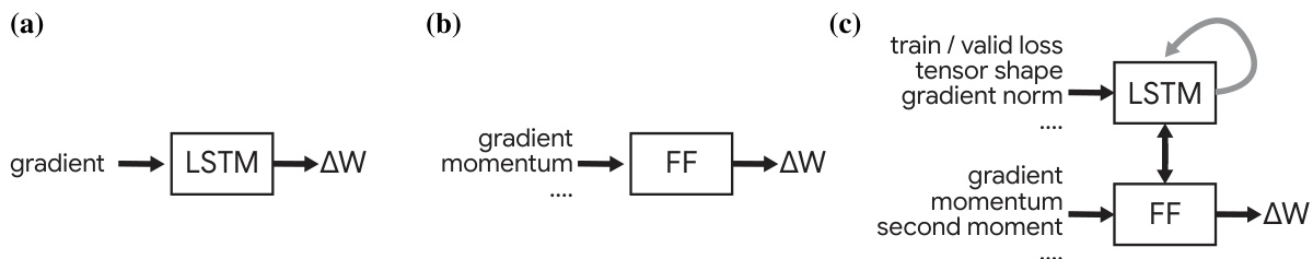
Figure 1: (a) The learned optimizer architecture proposed in An dry ch owicz et al. [9] consisting of a per-parameter LSTM. (b) The learned optimizer architecture proposed in Metz et al. [14] consisting of a per-parameter fully connected (feed-forward, FF) neural network with additional input features. (c) The learned optimizer architecture proposed in this work consisting of a per-tensor LSTM which exchanges information with a per-parameter feed forward neural network (FF). The LSTMs associated with each tensor additionally share information with each other (shown in gray).
图 1: (a) Andrychowicz等人[9]提出的学习优化器架构,包含一个逐参数的LSTM。(b) Metz等人[14]提出的学习优化器架构,包含一个带有额外输入特征的逐参数全连接(前馈,FF)神经网络。(c) 本工作提出的学习优化器架构,包含一个与逐参数前馈神经网络(FF)交换信息的逐张量LSTM。每个张量关联的LSTM还会相互共享信息(如灰色部分所示)。
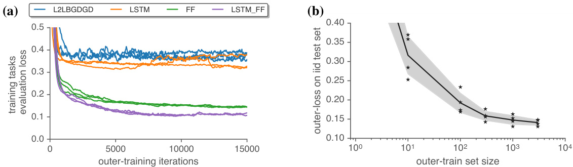
Figure 2: (a) Our proposed learned optimizer has a greater sample efficiency than existing methods. On the $\mathbf{X}$ -axis we show outer-updates performed to outer-train each learned optimizer. On the y-axis we show outer-loss. Each point consists of using a single outer parameter value to train 100 models for $10\mathrm{k\Omega}$ inner-iterations, each with five random initialization s. We show the average validation performance post-normalization averaged over all tasks, seeds, and inner-training steps. (b) Outergeneralization performance increases with an increasing number of outer-training tasks. We show the mean performance achieved after ${\sim}10000$ outer-training iterations (between 10500 and 9500) averaged over four random seeds while varying outer training set size. We show each seed as a star, and standard deviation as the shaded region. We find poor outer-generalization for smaller numbers of tasks. As we increase the number of outer-training tasks performance becomes more consistent, and lower loss values are achieved.
图 2: (a) 我们提出的学习优化器比现有方法具有更高的样本效率。横轴( $\mathbf{X}$ )表示对每个学习优化器进行的外部训练更新次数,纵轴表示外部损失。每个数据点代表使用单一外部参数值训练100个模型进行 $10\mathrm{k\Omega}$ 次内部迭代,每个模型采用五种随机初始化。图中显示的是所有任务、随机种子和内部训练步骤后经归一化的平均验证性能。(b) 外部泛化性能随外部训练任务数量的增加而提升。我们展示了在 ${\sim}10000$ 次外部训练迭代(介于10500至9500之间)后达到的平均性能,该结果是针对不同规模的外部训练集在四个随机种子上的平均值。每个种子以星号标记,阴影区域表示标准差。我们发现任务数量较少时外部泛化性能较差,随着外部训练任务数量的增加,性能表现更加稳定且能达到更低的损失值。
For per-parameter features we leverage effective inductive biases from hand-designed optimizers, and use a variety of features including the gradient, the parameter value, and momentum-like running averages of both. All features are normalized, in a fashion similar to that in RMSProp [30], or relative to the norm across the full tensor. For per-tensor features we use a variety of features built from summary statistics computed from the current tensor, the tensor’s gradient, and running average features such as momentum and second moments. We also include information about the tensor’s rank and shape. We also feed global features into the per-tensor LSTM, such as training loss and validation loss, normalized so as to have a relatively consistent scale across tasks. To compute a weight update, the per-parameter MLP outputs two values, $(a,b)$ , which are used to update inner-parameters: $\dot{w}^{t+1}=w^{\dot{t}}+\dot{\exp}(a)b$ . See Appendix C for many more details.
对于每个参数的特征,我们借鉴了手工设计优化器的有效归纳偏置,并使用了包括梯度、参数值以及两者的动量式滑动平均值在内的多种特征。所有特征都按照类似RMSProp [30] 的方式进行归一化,或相对于整个张量的范数进行归一化。对于每个张量的特征,我们使用了基于当前张量、张量梯度以及动量、二阶矩等滑动平均特征的多种统计摘要特征。我们还包含了张量的秩和形状信息。此外,我们将全局特征(如训练损失和验证损失)输入到每个张量的LSTM中,这些特征经过归一化处理,以保持跨任务间相对一致的尺度。为了计算权重更新,每个参数的多层感知机(MLP)输出两个值$(a,b)$,用于更新内部参数:$\dot{w}^{t+1}=w^{\dot{t}}+\dot{\exp}(a)b$。更多细节详见附录C。
4 Results
4 结果
4.1 Comparing learned optimizer architectures and training task set sizes
4.1 比较学习优化器架构与训练任务集规模
First, we show experiments comparing the performance of different learned optimizer architectures from the literature. We trained: a component-wise LSTM optimizer from An dry ch owicz et al. [9] (L2LBGDGD), a modification of this LSTM with the decomposed direction and magnitude output from Metz et al. [14] (LSTM), the fully connected optimizer from Metz et al. [14] (FF), as well as the proposed learned optimizer in this work (§3.3) (LSTM_FF). As shown in Figure 2(a), the proposed architecture achieves the lowest outer-training loss and achieves this in the fewest outer-training steps. To the best of our knowledge, this is the first published comparison across different learned optimizer architectures, on the same suite of tasks. Previous work only compared a proposed learned optimizer against hand-designed (baseline) optimizers.
首先,我们展示了比较文献中不同学习优化器架构性能的实验。我们训练了:来自Andrychowicz等人[9]的组件级LSTM优化器(L2LBGDGD)、Metz等人[14]对该LSTM的分解方向与幅度输出改进版本(LSTM)、Metz等人[14]的全连接优化器(FF),以及本文提出的学习优化器(§3.3)(LSTM_FF)。如图2(a)所示,所提架构实现了最低的外部训练损失,且以最少的外部训练步数达成目标。据我们所知,这是首次在同一套任务上对不同学习优化器架构进行公开比较。先前工作仅将提出的学习优化器与人工设计(基线)优化器进行对比。
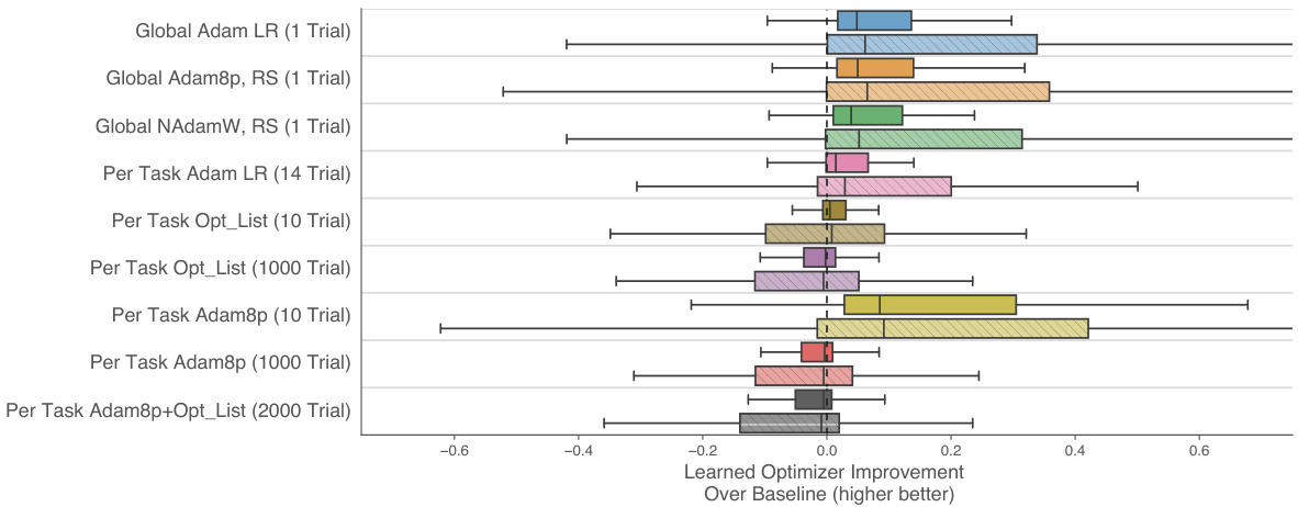
Figure 3: Learned optimizer performance as compared to a battery of different baselines. For each baseline, we show a box plot over 100 different tasks. We show both a training set (solid color) which the optimizer has seen, and a test set (hatched light color) which is sampled from the same distribution but never used for outer-training. Values to the right of the dashed line indicate the learned optimizer outperforming the corresponding baseline. The learned optimizer outperforms any single baseline optimizer with a fixed hyper parameter configuration (marked global, with a single Trial). We also outperform per-task tuning of baselines, when tuning is done only over a modest number of hyper parameter configurations (for instance, learning rate tuned Adam which uses 14 trials). Note that the learned optimizer undergoes no per-task tuning and only makes use of one trial.
图 3: 学习优化器与多种基线方法的性能对比。针对每个基线方法,我们展示了在100个不同任务上的箱线图。其中实色部分表示优化器已见过的训练集,浅色斜纹部分表示从相同分布采样但未用于外部训练的测试集。虚线右侧数值表示学习优化器优于对应基线方法的表现。该学习优化器在固定超参数配置下(标记为global,仅使用单次试验)超越了所有单一基线优化器。即使基线方法进行适度超参数调优(例如使用14次试验调整学习率的Adam),学习优化器仍表现更优。需注意学习优化器未进行任何任务级调优且仅使用单次试验。
Next, we explored how increasing the number of inner-tasks used when training an optimizer affects final performance. To do this, we randomly sampled subsets of tasks from the full task set, while evaluating performance on a common held-out set of tasks. Figure 2(b) shows that increasing the number of tasks leads to large improvements.
接下来,我们探究了在训练优化器时增加内部任务数量如何影响最终性能。为此,我们从完整任务集中随机抽取任务子集,同时在统一的保留任务集上评估性能。图2(b)显示,增加任务数量会带来显著提升。
4.2 Comparisons with hand-designed optimizers
4.2 与人工设计优化器的对比
We compare against three baseline optimizers: AdamLR, which is the Adam optimizer [31] with a tuned learning rate. Adam8p, which is a version of the Adam optimizer with eight tunable hyper parameters: learning rate, $\beta_{1}$ , $\beta_{2}$ , and $\epsilon$ , plus additional $\ell_{1}$ and $\ell_{2}$ regular iz ation penalties, and a learning rate schedule parameterized with a linear decay and exponential decay. See Appendix D for more details. Our final baseline optimizer, called opt_list, consists of the NAdam optimizer [32] with “AdamW” style weight decay [33], cosine learning rate schedules [34] and learning rate warm up (See Metz et al. [16] for more info). Instead of tuning these with some search procedure, however, we draw them from a sorted list of hyper parameters provided by [16] for increased sample efficiency.
我们对比了三种基线优化器:AdamLR,即经过学习率调优的Adam优化器[31];Adam8p,这是一种具有八个可调超参数的Adam优化器变体,包括学习率、$\beta_{1}$、$\beta_{2}$和$\epsilon$,以及额外的$\ell_{1}$和$\ell_{2}$正则化惩罚项,还有采用线性衰减和指数衰减参数化的学习率调度方案(详见附录D)。我们的最终基线优化器opt_list,由NAdam优化器[32]结合"AdamW"风格权重衰减[33]、余弦学习率调度[34]以及学习率预热组成(更多信息参见Metz等人[16])。不过,我们并非通过搜索过程来调整这些参数,而是从[16]提供的排序超参数列表中抽取,以提高样本效率。
Evaluation of optimizers, let alone learned optimizers, is difficult due to different tasks of interest, hyper parameter search strategies, and compute budgets [5, 35]. We structure our comparison by exploring two scenarios for how a machine learning practitioner might go about tuning the hyperparameters of an optimizer. First, we consider an “off-the-shelf” limit, where a practitioner performs a small number of optimizer evaluations using off-the-shelf methods (for instance, tuning learning rate only). This is typically done during exploration of a new machine learning model or dataset. Second, we consider a “finely tuned” limit, where a practitioner has a large compute budget devoted to tuning hyper parameters of a traditional optimizer for a particular problem of interest.
优化器(包括学习型优化器)的评估十分困难,这源于目标任务的差异性、超参数搜索策略的多样性以及计算资源的限制 [5, 35]。我们通过模拟机器学习实践者调整优化器超参数的两种典型场景来构建对比框架:
- 开箱即用模式:实践者仅使用现成方法(例如仅调整学习率)进行少量优化器评估。这种模式常见于探索新机器学习模型或数据集时。
- 精细调参模式:实践者为特定问题投入大量计算资源,专门用于传统优化器的超参数调优。
For the “off-the-shelf” limit, we consider the scenario where a practitioner has access to a limited number of optimization runs (trials) $(\leq10)$ for a particular problem. Thus, we select a first set of baseline hyper parameters using a single, default value (denoted global in Fig 3) across all of the tasks. We use random search (RS) using 1000 different hyper parameter values to find the global value that performs best on average for all tasks.
对于"现成可用"的限制,我们考虑实践者针对特定问题只能进行有限次数优化运行(试验) $(\leq10)$ 的场景。因此,我们首先选择一组基线超参数,在所有任务中使用单一默认值(图3中标记为global)。通过随机搜索(RS)使用1000组不同超参数值,找出在所有任务上平均表现最佳的全局值。
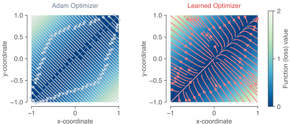
Figure 4: Implicit regular iz ation in the learned optimizer. Panels show optimization trajectories over a 2D loss surface, $\begin{array}{r}{f(x,y)=\frac{1}{2}\left(x-y\right)^{2}}\end{array}$ , that has a continuum of solutions along the diagonal. Left: Trajectories of the Adam optimizer go to the nearest point on the diagonal. Right: Trajectories of the learned optimizer go towards the diagonal, but also decay towards a single solution at the origin, as if there were an added regular iz ation penalty on the magnitude of each parameter.
图 4: 学习型优化器中的隐式正则化。面板展示了在二维损失曲面上的优化轨迹,该曲面函数为$\begin{array}{r}{f(x,y)=\frac{1}{2}\left(x-y\right)^{2}}\end{array}$,沿对角线存在连续解。左图:Adam优化器的轨迹收敛至对角线上最近点。右图:学习型优化器的轨迹不仅趋向对角线,还会衰减至原点处的单一解,仿佛对每个参数幅度施加了额外的正则化惩罚。
Practitioners often tune models with a small number of evaluations. As such, we include comparisons to per-task tuned learning rate tuned Adam, the first 10 entries of opt_list, and 10 hyper parameter evaluations obtained from random search using the adam8p hyper par meter iz ation.
从业者通常只需少量评估就能完成模型调优。为此,我们纳入了以下对比项:针对各任务单独调优的学习率Adam优化器、opt_list前10个配置项,以及通过adam8p超参空间随机搜索获得的10组超参评估结果。
For the “finely tuned” limit, we consider task-specific hyper parameter tuning, where the hyperparameters for each baseline optimizer are selected individually for each task (denoted per-task in Fig 3).
对于"精细调优"的极限情况,我们考虑任务特定的超参数调优,其中每个基线优化器的超参数会针对每个任务单独选择(在图3中标记为per-task)。
We plot a histogram over tasks showing the difference in performance between the each baseline optimizer and the learned optimizer in each row of Fig 3. First, we note that the distribution is broad, indicating that for some tasks the learned optimizer is much better, whereas for others, the baseline optimizer(s) are better. On average, we see small but consistent performance improvements over baseline optimizers, especially in the “off-the-shelf” scenario. We attribute this to the diverse set of tasks used for training the learned optimizer.
我们绘制了任务性能差异的直方图,展示图3每一行中基线优化器与学习优化器之间的表现差异。首先,我们注意到分布范围较广,这表明对于某些任务,学习优化器表现更优,而对于其他任务,基线优化器表现更好。平均而言,我们看到学习优化器相比基线优化器有微小但持续的性能提升,尤其是在"开箱即用"场景中。我们将此归因于用于训练学习优化器的多样化任务集。
4.3 Understanding optimizer behavior
4.3 理解优化器行为
To better understand the behavior of the learned optimizer, we performed probe experiments where we compared trajectories of the learned optimizer on simple loss surfaces against baseline optimizers. The goal of these experiments was to generate insight into what the learned optimizer has learned.
为了更好地理解所学优化器的行为,我们进行了探针实验,将所学优化器在简单损失曲面上的轨迹与基线优化器进行比较。这些实验的目的是深入了解所学优化器学到了什么。
In machine learning, many problems benefit from including some kind of regular iz ation penalty, such as an $\ell_{2}$ penalty on the weights or parameters of a model. We explored whether the learned optimizer (which was trained to minimize validation loss) had any implicit regular iz ation, beyond what was specified as part of the loss. To test this, we ran optimizers on a simple 2D loss surface, with a continuum of solutions along the diagonal: $\begin{array}{r}{f(x,y)=\frac{1}{2}\left(x-y\right)^{2}}\end{array}$ . Although any point along the $x=y$ diagonal is a global minimum, we wanted to see if the learned optimizer would prefer any particular solution within that set.
在机器学习中,许多问题都能通过引入某种正则化 (regularization) 惩罚项而受益,例如对模型权重或参数施加 $\ell_{2}$ 惩罚。我们探究了学习型优化器(训练目标是最小化验证损失)是否具有超出损失函数指定范围之外的隐式正则化。为此,我们在一个简单的二维损失曲面上测试优化器,该曲面沿对角线存在连续解集:$\begin{array}{r}{f(x,y)=\frac{1}{2}\left(x-y\right)^{2}}\end{array}$。虽然 $x=y$ 对角线上的任意点都是全局最小值,但我们希望观察学习型优化器是否会偏好该解集中的特定解。
Figure 4 shows the resulting training trajectories along the 2D loss surface from many starting points. For a baseline optimizer (left), the trajectories find the nearest point on the diagonal. However, we find that the learned optimizer has learned some implicit regular iz ation, in that it pushes the parameters towards a solution with small norm: $(0,0)$ .
图 4: 展示了从多个起点出发沿二维损失面的训练轨迹。对于基线优化器(左图),轨迹会找到对角线上最近的点。然而,我们发现学习到的优化器已掌握某种隐式正则化(regularization),它会将参数推向范数较小的解: $(0,0)$。
4.4 Generalization along different task axes
4.4 不同任务轴上的泛化能力
Next, we wondered whether the learned optimizer was capable of training machine learning models which differed across different architectural and training hyper parameters. To test this type of generalization, we trained fully connected neural networks on CIFAR-10 and MNIST, and swept three model hyper parameters: the number of hidden units per layer (network width), the batch size, and the number of training examples (dataset size, formed by sub sampling the full dataset). For each sweep, we compare the learned optimizer to a baseline optimizer, Adam, over a grid of eight different learning rates logarithmic ally spaced from $10^{-5.5}$ to $10^{^{\bullet}-2}$ .
接下来,我们想知道学习到的优化器是否能够训练在不同架构和训练超参数上存在差异的机器学习模型。为了测试这种泛化能力,我们在CIFAR-10和MNIST上训练全连接神经网络,并调整了三个模型超参数:每层隐藏单元数(网络宽度)、批量大小和训练样本数量(数据集大小,通过对完整数据集进行子采样形成)。对于每次调整,我们将学习到的优化器与基线优化器Adam在8个不同学习率的网格上进行比较,这些学习率在$10^{-5.5}$到$10^{^{\bullet}-2}$之间对数均匀分布。
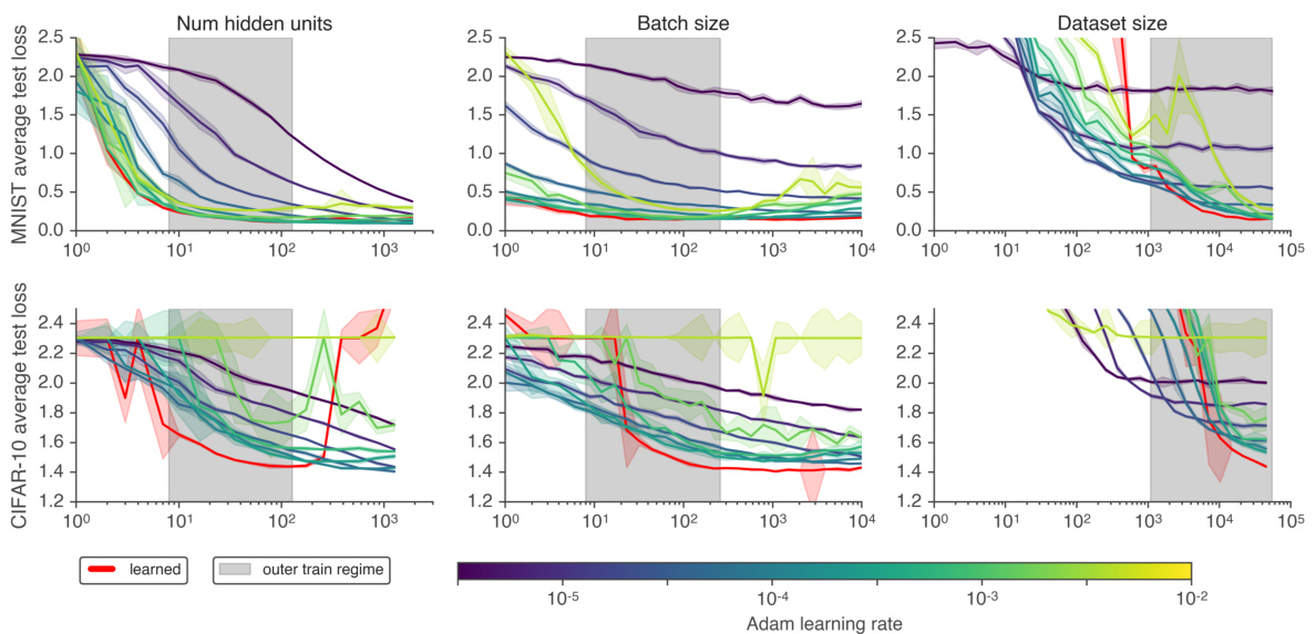
Figure 5: We show outer-generalization of the learned optimizer in a controlled setting by varying hyper parameters of the task being trained. We vary parameters around two types of models. Top row: A two hidden layer, 32 unit fully connected network trained on MNIST with batch size 128. Bottom row: A two layer hidden layer, 64 unit fully connected network trained on CIFAR-10 with batch size 128. We vary the width of the underlying network, batch size, and dataset size in each column. Each point on each curve shows the mean test loss averaged over 10k inner steps. We show median performance over five random task initialization s. Error bars denote one standard deviation away from the median. Color denotes different learning rates for Adam log spaced every half order of magnitude for Adam with purple representing $10^{-\overleftarrow{6}}$ , and yellow at $10^{-2}$ . We find the learned optimizer is able to generalize outside of the outer-training distribution (indicated by the shaded patch) in some cases.
图 5: 我们通过调整训练任务的超参数,在受控环境中展示所学优化器的外推泛化能力。实验围绕两类模型展开参数变化。上图: 在MNIST数据集上训练的批量为128的双隐藏层全连接网络(每层32单元)。下图: 在CIFAR-10数据集上训练的批量为128的双隐藏层全连接网络(每层64单元)。各列分别展示了基础网络宽度、批量大小和数据集规模的变动情况。曲线上的每个点表示1万次内部步骤的平均测试损失,数据点为五次随机任务初始化的中位数表现,误差条表示偏离中位数一个标准差。颜色代表Adam优化器的不同学习率(以半数量级对数间隔),紫色对应$10^{-\overleftarrow{6}}$,黄色对应$10^{-2}$。研究发现,所学优化器在某些情况下能够泛化至外训练分布之外(阴影区域标示)。
The results of these experiments are in Fig. 5. As we vary the number of hidden units (left column) or batch size (middle column), the learned optimizer generalizes outside of the range of hidden units used during training (indicated by the shaded regions). In addition, the learned optimizer matches the performance of the best learning rate tuned Adam optimizer. On CIFAR-10, as we move further away from the outer-training task distribution, the learned optimizer diverges. For dataset size (right column), we find that the learned optimizer is more sensitive to the amount of data present (performance drops off more quickly as the dataset size decreases). These experiments demonstrate the learned optimizer is capable of adapting to some aspects of target tasks which differ from its outer-training distribution, without additional tuning.
这些实验结果见图5。当我们改变隐藏单元数量(左列)或批处理大小(中列)时,学习到的优化器能够泛化到训练时所用隐藏单元范围之外(阴影区域所示)。此外,学习到的优化器性能与经过最佳学习率调优的Adam优化器相当。在CIFAR-10数据集上,当我们进一步偏离外部训练任务分布时,学习到的优化器会出现发散。对于数据集规模(右列),我们发现学习到的优化器对数据量更为敏感(随着数据集规模减小,性能下降更快)。这些实验表明,学习到的优化器能够在无需额外调优的情况下,适应目标任务中某些与外部训练分布不同的方面。
4.5 Generalization to large-scale problems
4.5 大规模问题的泛化
We test the learned optimizer on large-scale machine learning tasks. We use two ResNet V2 [36] architectures: a 14 layer residual network trained on CIFAR-10 [37]; and a 35 layer residual network trained on 64x64 resized ImageNet [38]. We train both networks with the learned optimizer and compare the performance to learning rate tuned Adam and Momentum (Fig. 6). Details in Appendix D. For CIFAR-10, we find that the learned optimizer achieves similar performance as the baselines but does not overfit later in inner-training. For ImageNet, we find that the learned optimizer performs slightly worse.
我们在大型机器学习任务上测试了所学优化器。采用两种ResNet V2 [36]架构:在CIFAR-10 [37]上训练的14层残差网络;以及在64x64尺寸调整后的ImageNet [38]上训练的35层残差网络。使用所学优化器训练这两个网络,并与学习率调优的Adam和Momentum进行性能对比(图6)。具体细节见附录D。对于CIFAR-10,我们发现所学优化器取得了与基线相当的性能,但在内部训练后期没有出现过拟合。对于ImageNet,所学优化器表现略逊一筹。
Note that our baselines only include learning rate tuning. More specialized hyper parameter configurations, designed specifically for these tasks, such as learning rate schedules and data augmentation strategies will perform better. An extensive study of learned optimizer performance on a wide range of state-of-the-art models is a subject for future work.
需要注意的是,我们的基线仅包含学习率调优。针对这些任务专门设计的更专业化的超参数配置(例如学习率调度策略和数据增强方案)将获得更优表现。关于学习优化器在各类前沿模型上的性能表现,仍需通过未来工作展开全面研究。
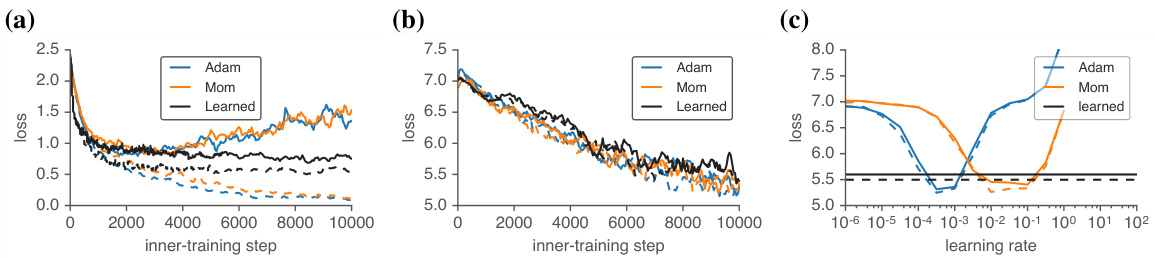
Figure 6: Learned optimizers are able to optimize ResNet models. (a) Inner-learning curves using the learned optimizer to train a small ResNet on CIFAR-10. We compare to learning rate tuned Adam and Momentum. Solid lines denote test performance, dashed lines are train. (b) Inner-learning curves using the learned optimizer to train a small ResNet on 64x64 resized ImageNet. We compare to learning rate tuned Adam and Momentum. (c) Performance averaged between $9.5\mathrm{k}$ and $10\mathrm{k\Omega}$ inner-iterations for Adam and Momentum as a function of learning rate, on the same task as in (b). Despite requiring no tuning, the learned optimizer performs similarly to these baselines after tuning.
图 6: 学习型优化器能够优化ResNet模型。(a) 使用学习型优化器在CIFAR-10上训练小型ResNet的内部学习曲线。我们与学习率调优后的Adam和Momentum进行比较。实线表示测试性能,虚线表示训练性能。(b) 使用学习型优化器在64x64尺寸调整后的ImageNet上训练小型ResNet的内部学习曲线。我们与学习率调优后的Adam和Momentum进行比较。(c) Adam和Momentum在$9.5\mathrm{k}$至$10\mathrm{k\Omega}$内部迭代区间内的平均性能(作为学习率的函数),任务设置与(b)相同。尽管无需调参,学习型优化器在调优后表现与这些基线方法相当。
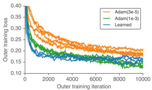
Figure 7: The learned optimizers can be used to train themselves about as efficiently as hand designed methods. On the $\mathbf{X}$ -axis we show number of weight updates done to the learned optimizer. On the y-axis we show outer-loss. Each point consists of inner-training 100 models, each with five random initialization s trained for 10k inner-iterations. We show the average validation performance post-normalization averaged over all tasks, seeds, and inner-training steps. Each line represents a different randomly initialized learned optimizer. In orange we show Adam with a learning rate of 3e-5 the same value used to train the optimizers in this work. In green, we show Adam with a learning rate of 1e-3, the learning rate that performed best in this 10k outer-iteration regime. In blue we show our learned optimizer.
图 7: 学习到的优化器能以与手工设计方法相当的效率训练自身。横轴( $\mathbf{X}$ )表示对学习优化器进行的权重更新次数,纵轴表示外部损失。每个数据点包含100个模型的内部训练,每个模型采用五次随机初始化并训练1万次内部迭代。图中显示的是所有任务、随机种子和内部训练步骤后归一化的平均验证性能。每条线代表不同随机初始化的学习优化器。橙色线表示学习率为3e-5的Adam(与本工作中训练优化器所用值相同),绿色线表示学习率为1e-3的Adam(在该1万次外部迭代机制中表现最佳),蓝色线表示我们学习到的优化器。
4.6 Learned optimizers training themselves
4.6 学习优化器的自我训练
Finally, we performed an experiment to test if a learned optimizer can be use to train new learned optimizers. Figure 8 shows that this “self-optimized” training curve is similar to the training curve using our hand-tuned training setup (using the Adam optimizer). We interpret this as evidence of unexpectedly effective generalization, as the training of a learned optimizer is unlike anything in the set of training tasks used to train the optimizer. We show outer-training for 10k outer-training iterations, matching the number of inner-iterations used when outer-training the learned optimizer. If outer-training is continued beyond $10\mathrm{k\Omega}$ iterations, learned optimizer performance worsens (see Appendix G), suggesting that more inner-iterations are needed when outer-training.
最后,我们进行了一项实验,测试学习到的优化器是否可用于训练新的学习优化器。图 8 显示,这种"自优化"训练曲线与使用手动调优训练设置(使用 Adam 优化器)的训练曲线相似。我们将此解释为意外有效泛化的证据,因为学习优化器的训练与用于训练该优化器的任务集中的任何内容都不同。我们展示了 10k 次外部训练迭代的外训练,与在学习优化器外训练时使用的内部迭代次数相匹配。如果外训练持续超过 $10\mathrm{k\Omega}$ 次迭代,学习优化器的性能会下降(见附录 G),这表明在外训练时需要更多的内部迭代。
5 Discussion
5 讨论
In this work, we train a learned optimizer using a larger and more diverse set of training tasks, better optimization techniques, an improved optimizer architecture, and more compute than previous work. The resulting optimizer outperforms hand-designed optimizers constrained to a single set of hyperparameters, and performs comparably to hand designed optimizers after a modest hyper parameter search. Further, it demonstrates some ability to generalize to optimization tasks unlike those it was trained on. Most dramatically, it demonstrates an ability to train itself.
在本工作中,我们使用比以往研究更大规模、更多样化的训练任务集、更优的优化技术、改进的优化器架构以及更强的算力来训练一个学习型优化器。最终得到的优化器性能优于使用固定超参数的手工设计优化器,并在经过适度超参数搜索后与手工优化器表现相当。此外,它展现出对训练任务之外优化问题的泛化能力。最显著的是,该优化器展示了自我训练的能力。
However, the learned optimizer we develop is not without limitations. Below we summarize areas for future work.
然而,我们开发的学习型优化器并非没有局限性。以下我们总结了未来工作的方向。
Generalization: While it performs well for tasks like those in TaskSet, we do not yet fully understand its outer-generalization capabilities. It shows promising ability to generalize to out of distribution problems such as training itself, and ResNet models, but it does not outperform competing algorithms in all settings on simple “out of distribution” optimization tasks, like those seen in Figure 5.
泛化性:虽然在TaskSet等任务上表现良好,但我们尚未完全理解其外部泛化能力。该系统在分布外问题上展现出有前景的泛化能力(例如对自身训练过程和ResNet模型的优化),但在简单"分布外"优化任务(如图5所示)中,其表现并未全面超越其他竞争算法。
Optimization / Compute: Currently it takes significant compute expenditure to train a learned optimizer at this scale, resulting in a nontrivial carbon footprint. Ideally training can be run once and the resulting learned optimizer can be used broadly as is the case with BERT [39].
优化/计算:目前在这个规模上训练一个学习到的优化器需要大量的计算开销,导致不小的碳足迹。理想情况下,训练可以只运行一次,然后像BERT [39]那样广泛使用所得到的学习优化器。
Learned optimizer architectures: We have shown there is considerable improvement to be had by incorporating better inductive biases both in outer-optimization speed and capacity. Improving these architectures, and leveraging additional features will hopefully lead to more performant learned optimizers. Additionally, the current optimizer, while compute efficient, is memory inefficient requiring $>5\times$ more storage per-parameter than Adam. We do not believe this poses a fundamental barrier, but modifications similar to those in Shazeer and Stern [40] will be needed to train larger models.
学习到的优化器架构:我们已经证明,通过在外层优化速度和容量方面融入更好的归纳偏置,可以带来显著提升。改进这些架构并利用额外特性,有望催生性能更优的学习型优化器。此外,当前优化器虽然计算效率高,但内存效率较低,每个参数所需的存储空间比Adam多$>5\times$倍。我们认为这并非根本性障碍,但要训练更大模型,需要采用类似Shazeer和Stern [40] 提出的改进方案。
Outer-training task distribution: We have shown that training on larger tasksets leads to better generalization. We have not studied which tasks should be included so as to aid outer-generalization.
外训练任务分布:我们已经证明在更大的任务集上进行训练能带来更好的泛化效果。但尚未研究应包含哪些任务以促进外泛化能力。
Acknowledgements
致谢
We would like to thank Alex Alemi, Eric Jang, Diogo Moitinho de Almeida, Timothy Nguyen, Alec Radford, Ruoxi Sun, Paul Vicol and Wojciech Zaremba for discussion related to this work as well as the Brain Team for providing a supportive research environment. We would also like to thank the authors of Numpy [41–43], Seaborn [44], and Matplotlib [45].
我们要感谢Alex Alemi、Eric Jang、Diogo Moitinho de Almeida、Timothy Nguyen、Alec Radford、Ruoxi Sun、Paul Vicol和Wojciech Zaremba就本工作进行的讨论,以及Brain Team提供的支持性研究环境。同时感谢Numpy [41-43]、Seaborn [44]和Matplotlib [45]的作者们。
Broader Impact
更广泛的影响
Machine learning training and inference is a major energy consumer, and training models likely dominates most individual machine learning researcher’s carbon emissions [46]. By meta-learning optimizers, we hope to amortize the cost of training ML models, and thus reduce the environmental impact of training a single model. We hope to achieve this both by reducing the need for extensive hyper parameter tuning as models are developed, and making training more efficient for the best hyper parameters.
机器学习训练与推理是主要的能源消耗环节,而模型训练很可能占据了大多数机器学习研究者个人碳排放的主要部分 [46]。通过元学习优化器,我们希望分摊训练ML模型的成本,从而降低单个模型训练对环境的影响。我们希望通过两方面实现这一目标:一是减少模型开发过程中大量超参数调优的需求,二是让最优超参数下的训练过程更加高效。
With this work, and more generally with meta-learning algorithms, we hope to provide researchers access to more performant easier to use optimizers for their problems. Improving technology to do machine learning will accelerate its impact, for better or worse. We believe machine learning technologies will be beneficial to humanity on the whole, and thus by improving the ability to optimize models we are moving towards this goal.
通过这项工作,以及更广泛的元学习算法,我们希望为研究人员提供性能更优、更易使用的优化器来解决他们的问题。提升机器学习相关技术将加速其影响力,无论好坏。我们相信机器学习技术总体上将对人类有益,因此通过提升模型优化能力,我们正朝着这一目标迈进。
Our optimizer is trained on a mixture of different tasks and datasets. It is our goal to construct an outer-training distribution that learns relevant inductive biases for machine learning tasks of interest. However, we currently do not have good methods to decipher exactly what types of inductive biases a learned optimizer might learn. Thus, future work is needed to explore what kinds of information is absorbed by learned optimizers. In the meantime, care should be taken when employing learned optimizers as the inductive biases of a particular learned optimizer may not be appropriate for an end user’s goals.
我们的优化器是在不同任务和数据集混合训练下完成的。我们的目标是构建一个外部训练分布,以学习相关机器学习任务所需的归纳偏置。然而,目前尚缺乏有效方法来精确解析已学习优化器可能习得的归纳偏置类型。因此,未来需要进一步探索学习型优化器吸收的信息种类。同时,在使用学习型优化器时应保持谨慎,因为特定优化器的归纳偏置可能与终端用户目标不匹配。
In fact, it has been suggested that learned optimizers could be a source of alignment drift in the development of Artificial General Intelligence (AGI) – leading to AGI that does not perform as its creators hoped [47]. While we do not feel that is an immediate danger from the present work, it is a consideration that should be kept in mind as learned optimizers become increasingly powerful.
事实上,有观点认为学习型优化器可能成为通用人工智能(AGI)发展过程中出现对齐漂移的诱因——导致AGI的行为偏离创造者的预期[47]。虽然我们认为当前研究尚未构成迫在眉睫的风险,但随着学习型优化器能力不断增强,这一潜在问题值得持续关注。
AExtended Related Work
扩展相关工作
We categorize progress in learned learned optimizers into three categories: parameter iz at ions, data distributions, and outer-training methodology. We include a review of these previous efforts herein.
我们将学习优化器的进展分为三类:参数化 (parameterizations)、数据分布 (data distributions) 和外层训练方法 (outer-training methodology)。本文对先前这些工作进行了综述。
A.1 Parameter iz at ions
A.1 参数化
Broadly, authors attack the problem of learned optimization at a high level using different parameterizations. We review these different choices below.
广义上,作者们从高层面对学习优化问题采用了不同的参数化方法进行攻克。我们将在下文回顾这些不同的选择。
A.1.1 Controller based parameter iz ation
A.1.1 基于控制器的参数化
One class of learned optimizer parameter ize s some function, usually as a neural network, that returns hyper parameters for an existing hand designed method. These methods impose a strong inductive bias. All inner-learning must be done via manipulation of existing methods. By enforcing a constrained structure, these method limit the types of learning rules expressible. This limitation does inject strong priors into the model making both outer optimization easier, as well as produce better outergeneralization. These methods often additionally make use off derived features from the currently training model. These features include things like loss values, variance of function evaluations, and variance of weight matrices.
一类学习优化器将某些函数(通常作为神经网络)参数化,用于返回现有手工设计方法的超参数。这些方法引入了强归纳偏置。所有内部学习必须通过对现有方法的操作来完成。通过强制约束结构,这些方法限制了可表达的学习规则类型。这种限制确实向模型注入了强先验,既使外部优化更容易,也产生了更好的外部泛化能力。这些方法通常还会利用当前训练模型派生的特征,包括损失值、函数评估方差和权重矩阵方差等指标。
There are a number of existing works that explore different types of features and architectures. Daniel et al. [6] explores using a simple, linear policy which maps from hand designed features to log learning rate which is then used with SGD, RMSProp or momentum. Xu et al. [7] learns a small LSTM network with inputs of current training loss, and predicts a learning rate for SGD. Xu et al. [8] uses an LSTM or an MLP with features computed during training and outputs a scalar which is multiplied by the previous learning rate.
现有研究探索了多种特征类型和架构。Daniel等人[6]采用简单的线性策略,将人工设计的特征映射为对数学习率,用于SGD、RMSProp或动量优化器。Xu等人[7]训练小型LSTM网络,以当前训练损失为输入,预测SGD的学习率。Xu等人[8]则使用LSTM或MLP架构,基于训练过程中计算的特征输出标量值,与先前学习率相乘。
A.1.2 Symbolic parameter iz at ions
A.1.2 符号参数化
Existing learning rules are often symbolic in nature. All first order optimizers used today are symbolic and expressible by a small collection of mathematical operations. Bello et al. [48] take inspiration from this and also parameter ize optimizers as collections of mathematical primitives. This parameter iz ation can lead to interpret able optimizers. For example, Bello et al. [48] show common sub patterns discovered based on multiplication of the sign of the gradient and sign of the momentum value. Not all computations lend themselves to a symbolic regression. Finding symbolic formula to solve increasingly more difficult tasks starts to resemble program synthesis which is notoriously difficult.
现有学习规则通常具有符号化特性。当前所有一阶优化器都是符号化的,可通过少量数学运算表达。Bello等人[48]受此启发,也将优化器参数化为数学原语的集合。这种参数化可产生可解释的优化器,例如[48]展示了基于梯度符号与动量值符号相乘所发现的常见子模式。但并非所有计算都适合符号回归——随着任务难度提升,寻找符号公式求解的过程会逐渐趋近于 notoriously difficult 的程序合成问题。
A.1.3 Continuous parameter iz at ions
A.1.3 连续参数化
The last family of parameter iz ation is based on continuously parameterized function approximations. Older work often makes use of simple / linear combinations of features while more recent work makes use of neural networks. There are a few classes of update rule parameter iz at ions.
最后一类参数化方法基于连续参数化的函数近似。早期研究常采用简单的特征线性组合,而近期工作则多使用神经网络。更新规则参数化可分为若干类别。
Bengio et al. [49] proposes a 7 parameter, and 16 parameter update rule parameterized by mixing various biologically inspired learning signals. Runarsson and Jonsson [50] use a simple continuous parameter iz ation that operates on error signals and produces changes in inner-parameters.
Bengio等人[49]提出了一种7参数和16参数更新规则,通过混合多种受生物学启发的学习信号进行参数化。Runarsson和Jonsson[50]采用了一种简单的连续参数化方法,基于误差信号操作并改变内部参数。
Recently, there has been renewed interest in learned optimizers, in particular using neural network para meri zat ions of the learning rules. An dry ch owicz et al. [9] makes use of an LSTM[25] possibly with global average pooling to enable concepts like $\ell_{2}$ gradient clipping to be implemented [51]. They also explore Neural Turing Machine [52] like parameter iz at ions specifically designed for low rank memory updates so that it can learn algorithms like LBFGS [53, 54]. In contrast, Metz et al. [14] makes use of a per-parameter MLP instead of the LSTM.
最近,人们对学习优化器重新产生了兴趣,特别是利用神经网络参数化学习规则。An dry ch owicz等人[9]采用了LSTM[25],可能结合全局平均池化,以实现诸如$\ell_{2}$梯度裁剪等概念的实现[51]。他们还探索了类似神经图灵机[52]的参数化方法,专门设计用于低秩内存更新,从而能够学习如LBFGS[53, 54]等算法。相比之下,Metz等人[14]则使用了针对每个参数的多层感知机(MLP)而非LSTM。
One critical design choice when designing neural network parameterized learned optimizers is input features. When training neural network models it is critical that the inputs be similar scales to aide in optimization. An dry ch owicz et al. [9] trains on raw gradients which are scaled by either decomposing each scalar into a sign and a magnitude before feeding into an LSTM. Lv et al. [11] uses the gradient and momentum normalized by the rolling average of gradients squared (similar to the rescaling done by Adam). Wichrowska et al. [10] also makes use of momentum except using multiple timescales normalized in a similar way. In addition to these momentum terms, Metz et al. [14] other features such as weight value and additionally applies a normalization based on the second moment of features.
设计神经网络参数化学习优化器时,一个关键的设计选择是输入特征。在训练神经网络模型时,确保输入具有相近的尺度以辅助优化至关重要。An dry ch owicz等人[9]采用原始梯度进行训练,通过将每个标量分解为符号和幅度后再输入LSTM进行缩放。Lv等人[11]使用梯度平方的滚动平均值对梯度和动量进行归一化(类似于Adam中的重缩放方法)。Wichrowska等人[10]同样利用了动量,但采用多时间尺度并按类似方式归一化。除了这些动量项外,Metz等人[14]还引入了权重值等特征,并基于特征的二阶矩应用了额外的归一化处理。
In [9, 11, 12] all methods employ a per-parameter update. The updates are independent of the number of parameters 1. While expressive, this is expensive as no computation can be shared. Wichrowska et al. [10] improve upon this by additionally having per-layer, and a global LSTM.
在[9, 11, 12]中,所有方法都采用了逐参数更新机制。这些更新与参数数量无关1。虽然表达能力强,但由于无法共享计算,这种方法成本高昂。Wichrowska等人[10]通过额外引入逐层更新和全局LSTM对此进行了改进。
When designing learned optimizer architectures, there are a number of design decisions to keep in mind. One must balance compute cost of the learned optimizer with express i bil it y. Often this shifts models to be considerably smaller than those used in supervised learning. Wichrowska et al. [10], for example makes use of a 8-hidden unit LSTM per-parameter. Selection of features to feed into the learned optimizer is also critical. While traditionally deep learning involves learning every feature, this learning comes at the cost of increased compute which is often not feasible.
在设计学习型优化器架构时,需考虑多项设计决策。开发者必须在学习型优化器的计算成本与表达能力之间取得平衡。这通常导致模型规模远小于监督学习所用的模型。例如 Wichrowska 等人 [10] 就采用了每参数 8 个隐藏单元的 LSTM 结构。选择输入学习型优化器的特征也至关重要:虽然传统深度学习会学习所有特征,但这种学习会带来难以承受的计算成本增长。
A.2 Data distribution of tasks
A.2 任务的数据分布
There is no agreed upon standards when defining datasets for training learned optimizers. The community is adhoc, training on what ever dataset is available or what ever best suites the goals (training a particular model, creating more general optimizers). Constructing large distributions of tasks is labor intensive and thus not often done.
在定义用于训练学习优化器的数据集时,目前尚无统一标准。该领域的研究具有临时性,通常基于现有数据集或最符合目标的数据集(如训练特定模型或开发更通用的优化器)进行训练。构建大规模任务分布需要大量人力,因此并不常见。
Metz et al. [14] draws inspiration from the few shot learning literature and constructs 10 way classification problems sampling from different classes on imagenet.
Metz et al. [14] 从少样本学习文献中汲取灵感,通过在 ImageNet 上对不同类别进行采样构建了 10 路分类问题。
Wichrowska et al. [10] leverages a large distribution of synthetic tasks. These tasks are designed to represent different types of loss surfaces that might be found in loss surfaces.
Wichrowska等人[10]利用了大量合成任务的分布。这些任务旨在代表损失曲面中可能出现的不同类型损失曲面。
TaskSet, [16] is a dataset of tasks specifically designed for learned optimizer research. We use this dataset throughout our work.
TaskSet [16] 是一个专为学习型优化器研究设计的任务数据集。我们在整个工作中都使用该数据集。
There is a balance between performance of the tasks, and ability to outer-train. Selecting the types of problems we want to train on is often not enough. Additionally, outer-training on the closest task possible will not produce the best optimizer nor even converge. Training on distributions with increased variation smooths the outer-loss surface and makes exploration simpler. This mirrors phenomena found in RL [55, 56].
在任务性能与外训练能力之间存在平衡。仅选择我们想要训练的问题类型往往不够。此外,在最接近的任务上进行外训练既不会产生最佳优化器,甚至无法收敛。在变化增大的分布上进行训练可以平滑外损失表面,使探索更简单。这与强化学习中发现的现象相呼应 [55, 56]。
A.3 Outer-Optimization methods
A.3 外部优化方法
The outer-optimization problem consists of finding a particular set of weights, or configuration of a learned optimizer. A number of different strategies have been proposed.
外层优化问题在于寻找一组特定的权重,或是学习优化器的某种配置。目前已有多种不同策略被提出。
A.3.1 Hyper parameter optimization
A.3.1 超参数优化
One of the most common outer-learning methods used is hyper-parameter optimization. In the context of learning optimizers, this can be seen as finding optimizer hyper parameters, e.g. learning rate, over a particular task instance. Numerous methods exist to do this ranging from Bayesian hyper parameter optimization [57], to grid search, to genetic algorithms. See Golovin et al. [58] for a more complete description.
最常用的外部学习方法之一是超参数优化。在学习优化器的背景下,这可以看作是为特定任务实例寻找优化器超参数(例如学习率)。实现这一目标的方法多种多样,包括贝叶斯超参数优化[57]、网格搜索和遗传算法等。更全面的描述可参考Golovin等人[58]的研究。
The types of outer-learning problems encountered in learned optimizers is different in that the evaluation function is often an expectation over some distribution. Additionally, the amount of outer-parameters is often larger than simply finding a few hyper parameters. Never the less, we include this here to show the similarity to learned optimizer research.
学习式优化器(learned optimizers)遇到的外部学习问题类型有所不同,其评估函数通常是某种分布的期望值。此外,外部参数量通常远超简单寻找几个超参数的情况。尽管如此,我们仍将其纳入讨论以展示其与学习式优化器研究的相似性。
A.3.2 Reinforcement learning
A.3.2 强化学习
Learned optimizers can naturally be cast into a sequential decision process. The state of the system consists of the inner-parameter values, action space is the steps taken, and the reward is achieving a low loss in the future. A number of works have thus taken this viewpoint. Li and Malik [59, 60] makes use of the guided policy search algorithm. Xu et al. [8] uses PPO Schulman et al. [61], Daniel et al. [6] make use of Relative Entropy Policy Search [62]. The exact algorithm used is a function of the underlying parameter iz ation.
学习型优化器自然可以被视为一个序列决策过程。系统状态由内部参数值构成,动作空间是采取的步骤,而奖励则是未来实现较低的损失。因此,多篇研究采用了这一视角。Li和Malik [59, 60] 利用了引导策略搜索算法。Xu等人 [8] 使用了PPO (Schulman等人 [61]),Daniel等人 [6] 则采用了相对熵策略搜索 [62]。具体使用的算法取决于底层参数化方式。
A.3.3 Neural Architecture Search Style
A.3.3 神经架构搜索风格
Instead of learning the policy directly, Bello et al. [48] makes use of reinforcement learning (PPO [61] to learn a controller which produces the symbolic learned optimizer. This is distinct from $\S\mathrm{A}.3.2$ as it does not leverage the sequential nature of the inner problem. Instead, it treats the environment as a bandit problem.
与直接学习策略不同,Bello等人[48]利用强化学习(PPO[61])训练控制器来生成符号化学习优化器。该方法与$\S\mathrm{A}.3.2$的区别在于:不利用内部问题的序列特性,而是将环境视为多臂老虎机问题。
A.3.4 Back pro pog ation / Gradient based
A.3.4 反向传播/基于梯度
Gradient based methods leverage local perturbations in parameter space. Computing derivatives through leaning procedures has been explored in the context of hyper parameter optimization in [63–65]. An dry ch owicz et al. [9] was the first to make use of gradient based learning for this application.
基于梯度的方法利用参数空间中的局部扰动。在超参数优化背景下,[63-65] 探讨了通过学习过程计算导数的方法。An dry ch owicz 等人 [9] 首次将基于梯度的学习应用于此场景。
To train a learned optimizer, ideally, one would compute the derivative of the entire training run with respect to optimizer parameters. This is often referred to as unrolling the entire training procedure into one large graph then running reverse mode automatic differentiation on this. Not only is this often too expensive to do in practice, the resulting loss surface can be poorly conditioned [14]. As such approximations are often made.
为了训练一个学习型优化器,理想情况下需要计算整个训练过程对优化器参数的导数。这通常被称为将整个训练过程展开成一个大图,然后对其运行反向模式自动微分。但这种方法不仅在实际中往往计算成本过高,而且得到的损失曲面可能条件不佳[14]。因此通常会采用近似方法。
One common family of approximation is based on truncated back pro pog ation through time. The core idea is to break apart long unrolled computations into shorter sequences and thus not propagating any error back through the entire unrolled computation graph pieces [66, 67]. This approximation is used widely in neural network parameterized learned optimizers [9–11, 14]. Unlike in language modeling, truncated backprop has been shown to lead to dramatically worse solutions for metalearning applications [19, 14].
一种常见的近似方法基于截断时间反向传播 (truncated back propagation through time)。其核心思想是将长时间展开的计算过程分解为较短的序列,从而避免误差在整个展开计算图中反向传播 [66, 67]。这种近似方法被广泛应用于神经网络参数化学习优化器 [9–11, 14]。与语言建模不同,研究表明截断反向传播会导致元学习应用的解决方案显著变差 [19, 14]。
A second family of approximations involve first order gradient calculations. An dry ch owicz et al. [9] does use the first order gradient calculation where as subsequent work, [10] does and computes the full gradient. The trade offs between these two gradient estimators has been discussed in the few shot learning literature in the context of MAML / Reptile [68, 69].
第二类近似方法涉及一阶梯度计算。An dry ch owicz等人[9]确实使用了一阶梯度计算,而后续工作[10]则计算完整梯度。这两种梯度估计器之间的权衡已在少样本学习文献中关于MAML/Reptile的背景下讨论过[68, 69]。
Computing gradients through iterative, non-linear, dynamics has been shown to cause chaotic dynamics. Pearl mutter [70], Maclaurin et al. [65] showed high sensitivity to learning rate with respect to performance after multiple steps of unrolled optimization. Metz et al. [14] shows this issue for neural network parameterized learned optimizers and proposes a solution based on variation al optimization and multiple gradient estimators.
通过迭代、非线性动力学计算梯度已被证明会导致混沌动力学。Pearl mutter [70] 和 Maclaurin 等人 [65] 研究表明,在展开多步优化后,性能对学习率具有高度敏感性。Metz 等人 [14] 针对神经网络参数化学习优化器揭示了这一问题,并提出基于变分优化和多重梯度估计器的解决方案。
Despite improvements, there are a lot of considerations that must be taken into account for doing gradient based training.
尽管有所改进,但基于梯度的训练仍需考虑诸多因素。
A.3.5 Evolutionary Strategies
A.3.5 进化策略
A alternative way to estimate gradients is to use black box method such as Evolutionary Strategies[71, 20, 72–74]. These methods are memory efficient, requiring no storage of intermediate states, but can suffer from high variance. In the case of learned optimizer optimization, however, these methods can result in lower variance gradient estimators [14]. Hybrid approaches that leverage both gradients and ES have been such as Guided ES [75] have also been proposed for meta-optimization. This work leverages one of the simplest forms of evolutionary strategies as described in [74] which uses a fixed standard deviation.
估计梯度的另一种方法是使用黑盒方法,如进化策略 (Evolutionary Strategies) [71, 20, 72–74]。这些方法内存效率高,无需存储中间状态,但可能存在高方差问题。然而,在学习优化器优化的情况下,这些方法可以产生方差更低的梯度估计器 [14]。同时,也有研究提出了结合梯度和进化策略的混合方法,例如用于元优化的引导进化策略 (Guided ES) [75]。本文采用了一种最简单的进化策略形式 [74],即使用固定标准差的方法。
B Outer Optimization Details
B 外部优化细节
In this work, as with Metz et al. [12], we use asynchronous, batched training. Each task has a different complexity, thus will produce outer-gradient estimates at a different rate. We use a syn crono us mini batched training as synchronous training with these he te rogen io us workloads would be too slow and wasteful. We tie the outer batch size to the number of workers. To prevent stale gradients, we additionally throw away all outer-gradient estimates that are from more than five outer-iterations away from the current weights.
在本工作中,与Metz等人[12]类似,我们采用异步批处理训练方式。由于每个任务具有不同复杂度,其产生外部梯度估计的速率也各不相同。我们采用同步小批量训练策略,因为针对这种异构工作负载进行完全同步训练会过于缓慢且低效。我们将外部批次大小与工作节点数量绑定。为防止梯度陈旧化,我们额外丢弃所有与当前权重相差超过五次外部迭代的梯度估计。
We optimize all models with Adam. We sweep learning rates between 3e-5 and 3e-3 for all experiments. We find the optimal learning rate is very sensitive and changes depending on how long outer-training occurs. We have preliminary explorations into learning rate schedules but have not yet been able to improve on this constant schedule. For all outer-training experiments, we always run more than one random seed. Due to the relatively small number of units, and biased gradient estimators, performance is dependant on random seed. For all experiments we use gradient clipping of 0.1 applied to each weight independently. Without this clipping no training occurs. This surprises us as our gradient estimator is evolutionary strategies which will not typically have exploding gradients. Upon further investigation, however, the outer-gradient variance is much larger without this clipping.
我们使用 Adam 优化所有模型。在所有实验中,我们将学习率扫描范围设定在 3e-5 至 3e-3 之间。我们发现最优学习率非常敏感,且会随外部训练时长而变化。我们初步探索了学习率调度方案,但尚未能改进这种固定调度方式。对于所有外部训练实验,我们始终运行多个随机种子。由于单元数量较少且梯度估计存在偏差,性能表现依赖于随机种子。所有实验均采用独立应用于每个权重的 0.1 梯度裁剪。若不进行裁剪,训练将无法进行。这让我们感到意外,因为我们的梯度估计采用的是通常不会出现梯度爆炸的进化策略。但进一步研究发现,若不进行裁剪,外部梯度的方差会显著增大。
When computing outer-gradients, we follow [14] and compute a outer-loss based on multiple mini batches of data. In our work we use 5. Note inner-training always uses a single minibatch of inner-training data as well as a single batch of inner-validation data when used.
计算外部梯度时,我们遵循[14]的方法,基于多个小批量数据计算外部损失。本工作中我们采用5个小批量。需注意,内部训练始终使用单个小批量的内部训练数据,若涉及内部验证数据时也仅使用单批次。
We first train with 240-360 length unrolls over a max of 10k inner-steps. While training we logged out 10k length unrolls from 100 tasks sampled from the outer-training distribution and saved outerparameters every hour. While training we monitor performance across all outer-learning rates and all seeds on the outer-training distribution. When training plateaus, we manually look through these evaluations and select a candidate set of optimizers to further train with an increasing truncation schedule. Not all optimizers fine tune in the same way despite having the same performance on the outer-training data so selecting more than one is critical. At this point we are unsure where this phenomenon comes from.
我们首先在最多1万次内部步骤上,使用240-360长度的展开进行训练。训练过程中,我们从外部训练分布中采样100个任务,记录1万长度的展开数据,并每小时保存一次外部参数。训练期间,我们会监控所有外部学习率和所有种子在外部训练分布上的表现。当训练进入平台期时,我们会手动检查这些评估结果,并选出一组候选优化器,采用逐步增加的截断计划继续训练。尽管在外部训练数据上表现相同,但并非所有优化器都以相同方式微调,因此选择多个优化器至关重要。目前我们尚不清楚这一现象的成因。
Next we fine tune theses models in an unbiased fashion. We explored two methods. First, based on an increasing truncation schedule. We tested linearly increasing truncation length from 300-10k steps over the course of $30\mathrm{k\Omega}$ or 10k steps. We find the faster increase, 10k steps, performs best. Second, we explored fine tuning with Persisted Evolutionary Strategies – an unbiased gradient estimator [21]. We found this achieved similar final performance but achieved it in half the time. When fine tuning we also make use of different learning rates. We find higher learning rates make progress faster, but can be unstable in that the performance varies as a function of outer-training step. Additionally, the learning rate chosen depends on the learning rate used previously in the first training phase. Before finetuning, we ‘warm up’ the Adam internal rolling statistics. While this might not be strictly required, it ensures that there is no decrease in performance early in outer-training. This can be done by simply setting the outer-learning rate to zero for the first 300 outer-iterations.
接下来我们以无偏方式对这些模型进行微调。我们探索了两种方法:第一种基于递增截断调度方案,测试了在$30\mathrm{k\Omega}$或1万步内将截断长度从300线性增加到1万步的情况,发现更快的1万步增幅方案效果最佳。第二种采用持久进化策略(Persisted Evolutionary Strategies)——一种无偏梯度估计器[21],发现该方法最终性能相当但耗时减半。微调时我们还采用了不同学习率,发现较高学习率能加速进程,但可能因外训练步数变化导致性能波动。此外,所选学习率取决于第一阶段训练采用的学习率。微调前会对Adam内部滚动统计量进行"预热",虽非必需但能避免外训练初期性能下降,具体实现只需在前300次外迭代中将外学习率设为零。
C Learned Optimizer Architecture Details
C 学习型优化器架构详解
In this section we describe the detailed learned optimizer architecture. For ease of understanding we opt to show a mix of pseudo-code based on python and textual descriptions as opposed to mathematical expressions. Finally we chose to describe our optimizer as a series of stateless and pure functions for clarity.
在本节中,我们将详细描述学习到的优化器架构。为了便于理解,我们选择展示基于Python语言的伪代码和文本描述的混合形式,而非数学表达式。最后,为了清晰起见,我们选择将优化器描述为一系列无状态且纯函数的形式。
We used this architecture for all of our experiments except of Fig 2b which used an older version of the architecture with additional features which where dropped from the final version.
除图 2b 使用了旧版架构(含最终版本已移除的附加功能)外,其余实验均采用此架构。
C.1 High level structure of the optimizer
C.1 优化器的高层结构
The learned optimizer has two main components: a function that maps from some set of inputs, a state, and parameters to some new state and new parameters.
学习到的优化器包含两个主要组件:一个将输入集、状态和参数映射到新状态和新参数的函数。
| class Optimizer: |
| def next_state(inputs: Inputs, |
| state: State, |
| parameters: Params |
| (State, Params); |
class Optimizer:
def next_state(inputs: Inputs,
state: State,
parameters: Params
(State, Params);
And a function to produce an initial state from the given inner-parameters.
以及一个根据给定内部参数生成初始状态的函数。
| def | initial_state(self, params: | Params) | -> | State; |
def initial_state(self, params: Params) -> State;
Parameters are stored as a dictionary of different tensors keyed by name.
参数以不同张量的字典形式存储,按名称索引。
For convenience, we also define gradients to be the same type as Params:
为方便起见,我们也将梯度定义为与Params相同的类型:
| Grads Params Dict [Text, Tensor] |
梯度参数字典 [Text, Tensor]
The state consists of multiple values that we will discuss in detail further. For now, however, we list the full state with high level comments.
状态由多个值组成,我们将在后文详细讨论。不过现在,我们先列出完整状态并附上概要说明。
State $=$ namedtuple ( " State ", [ # current inner training iteration " training step " : Int # the statistics for the rolling averages . " rolling features ": Rolling Feature State , # Hidden state of the lstm " l stm hidden state ": L STM Hidden State , # Activation s passed from the MLP to the LSTM. " from_mlp ": List [ Tensor [ shape $=$ ( from m lp size ,)]], # Activation s from LSTM passed to LSTM " from_lstm ": Tensor [ shape $=$ ( from l stm size ,)], # Rolling statistics of the train loss value " train loss ac cum ": Loss Ac cum State , # Rolling statistics of the valid loss value " valid loss ac cum ": Loss Ac cum State , # State to manage inner - gradinet clipping . " dynamic clip ": Rolling Clip State , # Parameter values from the nearest 100 steps in the past. ])
State = namedtuple( "State", [ # 当前内部训练迭代次数 "training_step": Int # 滚动平均的统计量 "rolling_features": RollingFeatureState, # LSTM的隐藏状态 "lstm_hidden_state": LSTMLSTMHiddenState, # 从MLP传递到LSTM的激活值 "from_mlp": List[Tensor[shape=(from_mlp_size,)]], # 从LSTM传递到LSTM的激活值 "from_lstm": Tensor[shape=(from_lstm_size,)], # 训练损失值的滚动统计量 "train_loss_accum": LossAccumState, # 验证损失值的滚动统计量 "valid_loss_accum": LossAccumState, # 内部梯度裁剪的管理状态 "dynamic_clip": RollingClipState, # 过去最近100步的参数值 ])
Both from l stm size, from m lp size are hyper parameters set as part of the learned optimizer to control how much information is sent from the MLP or from the LSTM.
从LSTM大小和MLP大小都是作为学习优化器的一部分设置的超参数,用于控制从MLP或LSTM发送的信息量。
The input to the next_state function consists of inner-gradients, computed on a inner-training batch of data, as well as optionally validation data which is passed in every 10 iterations. We choose to not pass in validation data every steps for computational efficiency.
next_state函数的输入包括在内部训练数据批次上计算得到的内部梯度 (inner-gradients) ,以及每10次迭代传入的可选验证数据。出于计算效率考虑,我们选择不每一步都传入验证数据。
Inputs $=$ namedtuple ( " Inputs ", [ # gradient from task. This is same type as the parameters . " inner grads ": Grads , # training loss computed from a mini batch . " train_loss ": float , # validation loss from a mini batch of validation data. " valid_loss ": Optional [ float ], ])
Inputs = namedtuple("Inputs", [ # 来自任务的梯度。与参数类型相同。 "inner_grads": Grads, # 通过小批量数据计算出的训练损失。 "train_loss": float, # 来自验证数据小批量的验证损失。 "valid_loss": Optional[float], ])
Each task specifies a function that samples parameter initialization, as well as to produce outputs.
每个任务指定一个用于采样参数初始化的函数,以及生成输出的函数。
class Task : def initial params ( self ) -> Params def inputs for params (self , params ) -> ( Grads , # inner - training gradients float , # inner - training loss Optional [ float ]) # optional inner - training validation
class Task : def initial params ( self ) -> Params def inputs for params (self , params ) -> ( Grads , # 内部训练梯度 float , # 内部训练损失 Optional [ float ]) # 可选的内部训练验证
For outer-training each task also includes a second loss function which computes the task’s loss on the outer-validation split of data. Note this uses a different validation set of data than the previous function.
对于外部训练,每个任务还包含第二个损失函数,用于计算该任务在外部分割验证数据上的损失。请注意,这里使用的验证数据集与前一个函数不同。
Inner training / application of the learned optimizer looks like:
学习优化器的内部训练/应用过程如下:
Computing the outer objective and outer-gradients from inner-initialization looks like the following:
从内部初始化计算外部目标和外部梯度的过程如下:
C.2 Utilities / components
C.2 实用工具/组件
First we will describe the individual components and utilities used, then we will go on to describe the full update function.
首先我们将介绍所使用的各个组件和工具,然后继续描述完整的更新函数。
C.2.1 Rolling Features
C.2.1 滚动特征
These are a moving average of gradients and second moments computed similarly to Adam / RMSProp. The rolling state consists of tensors containing momentum values (ms) and second moment values (rms):
这些是梯度和二阶矩的移动平均值,计算方式与 Adam/RMSProp 类似。滚动状态由包含动量值 (ms) 和二阶矩值 (rms) 的张量组成:
| RollingFeaturesState | collections.namedtuple("RollingFeaturesState" |
| ["ms":I Dict[Text,Tensor] | |
| rms Dict[Text, Tensor]]) |
| RollingFeaturesState | collections.namedtuple("RollingFeaturesState" |
|---|---|
| ["ms": Dict[Text, Tensor] | |
| rms Dict[Text, Tensor]) |
The Text represent names that map to the tensor of the corresponding shape from the parameters. The values are the same shape as the corresponding inner-parameter with an additional axis appended to keep track of multiple different decay values. While its possible to outer-learn these values, we fix them at 0.5, 0.9, 0.99, 0.999, 0.9999.
文本表示映射到参数中对应形状张量的名称。这些值与对应的内部参数形状相同,但额外增加了一个轴以跟踪多个不同的衰减值。虽然可以通过外部学习这些值,但我们将其固定为0.5、0.9、0.99、0.999、0.9999。
To update these we construct a helper class.
为了更新这些内容,我们构建了一个辅助类。
Class Rolling State : def init (self , decay values ): self . decay values $=$ decay values
类滚动状态: def init(self, decay values): self.decay values = decay values
We define an initial value which is simply simply zeros:
我们定义一个初始值,它简单地全为零:
def initial state (self , params : Params ): -> Rolling Feature State n_dims $=$ len( decay values )
初始状态 (self, params: Params): -> 滚动特征状态 n_dims $=$ len(decay values)
ms = {k: tf. zeros ([v. shape $^+$ [ n_dims ]} rms $=$ {k: tf. zeros ([v. shape + [ n_dims ]} return Rolling Features State ( ${\mathfrak{m}}\mathbf{s}={\mathfrak{m}}\mathbf{s}$ , rms = rms )
ms = {k: tf.zeros([v.shape $^+$ [n_dims]} rms $=$ {k: tf.zeros([v.shape + [n_dims]} return Rolling Features State (${\mathfrak{m}}\mathbf{s}={\mathfrak{m}}\mathbf{s}$, rms=rms)
To update these values we follow a procedure similar to RMSProp update equations:
为更新这些值,我们遵循与RMSProp更新方程类似的步骤:
def update state (self , state : Rolling Feature State , grads : Grads ) > Rolling Feature State : $\begin{array}{r c l}{{{\bf r}{\bf e}{\sf t}_ {-}{\sf m}{\bf s}}}&{{=}}&{{{\bf}}}\ {{{\bf r}{\bf e}{\bf t}_{-}{\bf r}{\bf m}{\bf s}}}&{{=}}&{{{\bf}}}\end{array}$ for k in state . keys (): ${\tt{g}}={\tt{\Psi}}$ grads [k] $\mathrm{~\bf~s~}=$ state [k] ret_ms [k] $=$ np. zeros_like (ret.ms[k]) ret_rms [k] $=$ np. zeros_like ( state .rms[k]) for di , decay in enumerate ( self . decay values ): ret_ms [k][... , di] $=$ ret[k][..., di] $^ * $ decay + (1 - decay ) * grad ret_rms [k][... , di] $=$ ret[k][.. di] $^ * $ decay $^+$ (1 decay ) $^*$ grad ** 2 return Rolling Feature State ( ${\mathfrak{m}}{\mathfrak{s}}={\mathfrak{r}}$ et_ms , rms $=$ ret_rms )
def update state (self , state : Rolling Feature State , grads : Grads ) > Rolling Feature State : $\begin{array}{r c l}{{{\bf r}{\bf e}{\sf t}_ {-}{\sf m}{\bf s}}}&{{=}}&{{{\bf}}}\ {{{\bf r}{\bf e}{\bf t}_{-}{\bf r}{\bf m}{\bf s}}}&{{=}}&{{{\bf}}}\end{array}$
for k in state . keys ():
${\tt{g}}={\tt{\Psi}}$
grads [k]
$\mathrm{~\bf~s~}=$
state [k]
ret_ms [k] $=$ np. zeros_like (ret.ms[k])
ret_rms [k] $=$ np. zeros_like ( state .rms[k])
for di , decay in enumerate ( self . decay values ):
ret_ms [k][... , di] $=$ ret[k][..., di] $^*$ decay + (1 - decay ) * grad
ret_rms [k][... , di] $=$ ret[k][.. di] $^*$ decay $^+$ (1 decay ) $^*$ grad ** 2
return Rolling Feature State ( ${\mathfrak{m}}{\mathfrak{s}}={\mathfrak{r}}$ et_ms , rms $=$ ret_rms )
C.2.2 LossAccum
C.2.2 LossAccum
This represents how we get loss information into our learned optimizer. Loss values have no predetermined scale and span many orders of magnitude. As such, we must somehow standardize them so that the inputs are bounded and able to be easily used by neural networks. We get around this by keeping track of the normalized mean and variance of the mini-batch losses.
这代表了我们如何将损失信息输入到学习到的优化器中。损失值没有预定的尺度,且跨越多个数量级。因此,我们必须以某种方式将其标准化,使得输入有界且易于神经网络使用。我们通过跟踪小批量损失的正态化均值和方差来解决这一问题。
Loss Ac cum State $=$ collections . namedtuple (" Loss Ac cum State ", [" mean ": float , # rolling mean loss value "var": float , # rolling second moment loss value " updates ": int # Number of updates performed so far ])
损失累积状态 (Loss Accum State) = collections.namedtuple("Loss Accum State", ["mean": float, # 滚动平均损失值 "var": float, # 滚动二阶矩损失值 "updates": int # 当前已执行的更新次数 ])
The class that manages these states is parameterized by the decay of the rolling window.
管理这些状态的类通过滚动窗口的衰减进行参数化。
class LossAccum : def init (self , decay ): self. decay $=$ decay
class LossAccum : def init (self , decay ): self. decay $=$ decay
The initial state is simply zeros.
初始状态全为零。
def initial state ( self ) -> Loss Ac cum State : return Loss Ac cum State ( mean $=$ tf. constant (0., dtype $=$ tf. float32 ), var $=$ tf. constant (0., dtype $=$ tf. float32 ), updates $=$ tf. constant (0, dtype $=$ tf. int64 ))
def initial state ( self ) -> Loss Ac cum State : return Loss Ac cum State ( mean $=$ tf. constant (0., dtype $=$ tf. float32 ), var $=$ tf. constant (0., dtype $=$ tf. float32 ), updates $=$ tf. constant (0, dtype $=$ tf. int64 ))
To compute updates we do rolling mean and variance computations.
为了计算更新,我们进行滚动均值和方差计算。
def next_state (self , state : Rolling Ac cum State , loss : float ): -> Loss Ac cum State new_mean $=$ self.decay $^ * $ state.mean $^+$ (1.0 - self. decay ) $^ * $ loss new_var $=$ self.decay $^ * $ state.var $^+$ ( 1.0 - self.decay) $^*$ tf. square ( new_mean - loss) new updates $=$ state . updates $^+\quad1$ return Loss Ac cum State ( mean $=$ new_mean , var $=$ new_var , updates $=$ new updates )
def next_state (self , state : Rolling Ac cum State , loss : float ): -> Loss Ac cum State new_mean $=$ self.decay $^ * $ state.mean $^+$ (1.0 - self. decay ) $^ * $ loss new_var $=$ self.decay $^ * $ state.var $^+$ ( 1.0 - self.decay) $^*$ tf. square ( new_mean - loss) new updates $=$ state . updates $^+\quad1$ return Loss Ac cum State ( mean $=$ new_mean , var $=$ new_var , updates $=$ new updates )
Two additional functions are used to normalize loss values for use in neural networks. First, we have a “corrected” mean (similar to what is done by Adam) for a given AccumState.
使用两个附加函数对损失值进行归一化处理,以便在神经网络中使用。首先,我们为给定的AccumState计算"修正"均值(类似于Adam优化器的做法)。
def corrected mean (self , state : AccumState ) -> float : c = 1. / (1 - self.decay $^{**}$ tf. to_float ( state . updates ) + 1e-8) return state . mean $^*$ c
def corrected_mean(self, state: AccumState) -> float:
c = 1. / (1 - self.decay$^{**}$ tf.to_float(state.updates) + 1e-8)
return state.mean$^*$ c
Second, we have a function that weights one loss by a different AccumState. This is eventually used to weight the validation loss accum against the training loss state allowing the learned optimizer to detect over fitting.
其次,我们有一个函数,它通过不同的 AccumState 对某个损失进行加权。这一机制最终用于对验证损失累积与训练损失状态进行加权,使学习到的优化器能够检测过拟合。
def weight loss (self , state : AccumState , loss : float ) -> float : $\textsf{c}=\textsf{1}$ . / (1 - self.decay $^{**}$ tf. to_float ( state . updates ) $^+$ 1e-8) cor_mean $=$ state.mean $^ * $ c cor_var $=$ state.var $^ * $ c $\begin{array}{r l}{{}^{1}}&{{}={}}\end{array}$ (loss - cor_mean ) $^*$ tf. rsqrt ( cor_var + 1e-8) return tf. clip by value (l, -5, 5)
def weight loss (self , state : AccumState , loss : float ) -> float : $\textsf{c}=\textsf{1}$ . / (1 - self.decay $^{**}$ tf. to_float ( state . updates ) $^+$ 1e-8) cor_mean $=$ state.mean $^ * $ c cor_var $=$ state.var $^ * $ c $\begin{array}{r l}{{}^{1}}&{{}={}}\end{array}$ (loss - cor_mean ) $^*$ tf. rsqrt ( cor_var + 1e-8) return tf. clip by value (l, -5, 5)
C.2.3 Rolling Clip State
C.2.3 滚动剪辑状态
Gradient clipping is a often used technique in deep learning. We found large benefits by applying some form of learned clipping (clipping inner-gradient values) in our learned optimizer. We cannot simply select a default value because gradient norms vary across problem. As such we meta-learn pieces of a dynamic gradient clipping algorithm. This is our first iteration of this concept and we expect large gains can be obtained with a better scheme.
梯度裁剪是深度学习中常用的技术。我们发现,在学习的优化器中应用某种形式的自适应裁剪(即裁剪内部梯度值)能带来显著优势。由于不同问题的梯度范数存在差异,我们无法简单地选择默认值。因此,我们通过元学习构建了动态梯度裁剪算法的关键组件。这是该概念的首次迭代,我们预期通过更优方案能实现更大提升。
This algorithm is stateful thus also needs some state container.
该算法是有状态的,因此也需要某种状态容器。
| RollingClipState | (int, | the | number | of | times | this | has | been | updated, | ||
| float | t# rolling | average | of | mean | of | squared | |||||
| gradient | values | ||||||||||
| RollingClipState | (int, | the | number | of | times | this | has | been | updated, | ||
|---|---|---|---|---|---|---|---|---|---|---|---|
| float | t# rolling | average | of | mean | of | squared | |||||
| gradient | values | ||||||||||
This class is parameterized by the decay constant of the rolling average and the multiplier to determine when clipping should start. Both of these values are outer-learned with the rest of the learned optimizer.
该类由滚动平均的衰减常数和确定何时开始剪裁的乘数参数化。这两个值与其他学习优化器一起进行外部学习。
| class RollingGradClip: def -_init_-(self, alpha=0.99, clip_mult=10): |
class RollingGradClip: def -init- (self, alpha=0.99, clip_mult=10):
The initial states are initialized to 1.
初始状态设为1。
def initial state ( self ) -> Rolling Clip State : return (tf. constant (1, dtype $=$ tf. float32 ), tf. constant (1.0, dtype $=$ tf. float32 )*(1- self . alpha ))
初始状态 (self) -> Rolling Clip State: return (tf.constant(1, dtype $=$ tf.float32), tf.constant(1.0, dtype $=$ tf.float32)*(1 - self.alpha)
We provide a normalization function that both updates the Rolling Clip State and provides clipped gradients.
我们提供了一个归一化函数,既能更新滚动裁剪状态,又能提供裁剪后的梯度。
def next state and normalize (self , state : Rolling Clip State , grads : Grads ) -> Rolling Clip State , Grads : def _normalize ( state $:$ Rolling Clip State , grads $:$ Grads ): summary ops $=[ ]$ t, snd $=$ state clip amount $=$ (snd / (1-self. alpha $^{\ast\ast}$ t)) $^*$ self . clip_mult clipgs $=$ [tf. clip by value (g, - clip amount , clip amount ) for g in grads . values ()] returnclipgs
def next state and normalize (self , state : Rolling Clip State , grads : Grads ) -> Rolling Clip State , Grads : def _normalize ( state $:$ Rolling Clip State , grads $:$ Grads ): summary ops $=[ ]$ t, snd $=$ state clip amount $=$ (snd / (1-self. alpha $^{\ast\ast}$ t)) $^*$ self . clip_mult clipgs $=$ [tf. clip by value (g, - clip amount , clip amount ) for g in grads . values ()] returnclipgs
C.3 Learned optimizer specific / putting it all together
C.3 学习优化器专项/整体整合
The learned optimizer has two main components. The first is the Optimizer class that manages everything surrounding inner-learning. This function has no learnable outer-parameters. The second is what we call “theta_mod” which contains all of the outer-variables and functions that we are learning.
学习到的优化器包含两个主要组件。第一个是Optimizer类,它负责管理所有与内部学习相关的事务。该函数没有可学习的外部参数。第二个是我们称为"theta_mod"的部分,它包含了我们正在学习的所有外部变量和函数。
First we construct the optimizer class with the corresponding theta_mod (see bellow).
首先我们构建带有相应 theta_mod 的优化器类 (参见下文)。
| class Optimizer: | |
| def | _init_-(self,theta_mod): |
| self.theta_mod | d=theta_mod |
class Optimizer:
def _init_- (self, theta_mod):
self.theta_mod = theta_mod
Next the rolling features at fixed, hard coded intervals. These could be outer-learned but in this work they are fixed.
接下来是在固定、硬编码间隔处的滚动特征。这些可以外部学习,但在本研究中它们是固定的。
self . rolling features $=$ Rolling Features ( decays $=$ [0.5, 0.9, 0.99 , 0.999 , 0. 9999 ])
self . rolling features $=$ 滚动特征 (decays $=$ [0.5, 0.9, 0.99, 0.999, 0.9999])
Then the the loss features for use with both training and validation loss. We use a lower decay constant on the validation as it is updated less frequently (once every 10 steps). Once again these could be outer-learned but in this work we leave them fixed.
随后是用于训练和验证损失的损失特征。由于验证损失更新频率较低(每10步一次),我们为其使用了较低的衰减常数。同样,这些参数也可以通过外部学习获得,但在本工作中我们将其固定不变。
| self.train_loss_accum LossAccum(0.95) self.valid_loss_accum LossAccum(o.9) |
self.train_loss_accum LossAccum(0.95) self.valid_loss_accum LossAccum(0.9)
Finally we construct the gradient clipping utility. Unlike the previous parameters, we do outer-learn these and pass in two variables off of the ‘theta_mod’.
最后我们构建梯度裁剪工具。与之前的参数不同,我们通过外部学习这些参数并传入两个来自 'theta_mod' 的变量。
| self.rolling_clip | RollingGradClip( |
| self.theta_mod.rolling_clip_alpha | |
| Self.theta_mod.rolling_clip_mult) |
| self.rolling_clip | RollingGradClip( |
|---|---|
| self.theta_mod.rolling_clip_alpha | |
| Self.theta_mod.rolling_clip_mult) |
Next, we need an initial state for the optimizer defined in C.1. This mostly consists of obtaining initial states from the various components of the learned optimizer.
接下来,我们需要为C.1节定义的优化器提供一个初始状态。这主要包括从学习优化器的各个组件中获取初始状态。
def initial State (self , params : Params ) -> State : shapes $=$ [v. shape . as_list () for v in params . values ()] return State ( training st $\mathtt{e p}=0$ , rolling features $=$ self . rolling features . initial state ( shapes ), from_lstm $=$ self . theta_mod . initial from l stm () , from_mlp $=$ self . theta_mod . initial from m lp ( len ( shapes )), l stm hidden stat $\ominus=$ self . theta_mod . initial rn n state ( len ( shapes ) ), train loss ac cum $=$ self . train loss ac cum . initial state () , valid loss ac cum $=$ self . valid loss ac cum . initial state () , dynamic clip $=$ self . rolling clip . initial state () , )
def initial State (self , params : Params ) -> State : shapes $=$ [v. shape . as_list () for v in params . values ()] return State ( training st $\mathtt{e p}=0$ , rolling features $=$ self . rolling features . initial state ( shapes ), from_lstm $=$ self . theta_mod . initial from l stm () , from_mlp $=$ self . theta_mod . initial from m lp ( len ( shapes )), l stm hidden stat $\ominus=$ self . theta_mod . initial rn n state ( len ( shapes ) ), train loss ac cum $=$ self . train loss ac cum . initial state () , valid loss ac cum $=$ self . valid loss ac cum . initial state () , dynamic clip $=$ self . rolling clip . initial state () , )
Next we look to the update performed. We split up into two components – first a validation state, and second a training state.
接下来我们关注所执行的更新。我们将其拆分为两个部分——首先是验证状态,其次是训练状态。
def next params and state (self , params : Params , current state : State , train_loss : float , train grads : Grads , valid_loss : Optional [ float ]) -> (Params , State ): if valid_loss : current state $=$ self . next state validation ( current state , valid_loss ) params , next_state $=$ self . next state train in ing ( params , current state , train_loss , train grads ) return params , next_state
def next params and state (self , params : Params , current state : State , train_loss : float , train grads : Grads , valid_loss : Optional [ float ]) -> (Params , State ): if valid_loss : current state $=$ self . next state validation ( current state , valid_loss ) params , next_state $=$ self . next state train in ing ( params , current state , train_loss , train grads ) return params , next_state
The validation update simply consists of updating the two components that make use of the loss value.
验证更新仅包括更新使用损失值的两个组件。
def next state validation (self , current state $:$ State , valid_loss : float ) -> State : next valid loss ac cum $=$ self . valid loss ac cum . next_state ( current state . valid loss ac cum , valid_loss ) return current state . _replace ( valid loss ac cum $=$ next valid loss ac cum )
def next_state_validation(self, current_state $:$ State, valid_loss: float) -> State:
next_valid_loss_accum $=$ self.valid_loss_accum.next_state(current_state.valid_loss_accum, valid_loss)
return current_state._replace(valid_loss_accum $=$ next_valid_loss_accum)
The the function applied to the training gradients is much more complicated. Much like the validation features it updates the various rolling statistics including the two loss data structures, the rolling momentum / rms terms, as well as the gradient clipping state.
应用于训练梯度的函数要复杂得多。与验证特征类似,它会更新各种滚动统计量,包括两个损失数据结构、滚动动量/RMS项以及梯度裁剪状态。
def next state train in ing (self , params : Params , current state : State , loss : float , grads : Grads ) -> (Params , State ): grads $=$ list ( grads . values ()) next train loss ac cum $=$ self . train loss ac cum . next_state ( current state . train loss ac cum , loss ) next dynamic clip , grads $=$ self . rolling clip . next state and normalize ( current state . dynamic clip , grads ) next rolling features $=$ self . rolling features . next_state ( current state . rolling features , grads )
def next_state_train_in_ing(self, params: Params, current_state: State, loss: float, grads: Grads) -> (Params, State):
grads = list(grads.values())
next_train_loss_accum = self.train_loss_accum.next_state(current_state.train_loss_accum, loss)
next_dynamic_clip, grads = self.rolling_clip.next_state_and_normalize(current_state.dynamic_clip, grads)
next_rolling_features = self.rolling_features.next_state(current_state.rolling_features, grads)
Next, a sequence of features related to loss values are computed.
接下来,计算一系列与损失值相关的特征。
Next we call into the learned optimizer function in “theta_mod” which does the bulk of the computation.
接下来我们调用学习到的优化器函数 "theta_mod",该函数承担了大部分计算工作。
next params , from_lstm , from_mlp , l stm hidden state $=$ self . theta_mod . compute update and next state ( train loss feat , valid loss feat , current state . from_mlp , current state . from_lstm , current state . l stm hidden state ,
下一个参数, from_lstm, from_mlp, lstm隐藏状态 $=$ self.theta_mod.compute_update_and_next_state(训练损失特征, 验证损失特征, current_state.from_mlp, current_state.from_lstm, current_state.lstm_hidden_state,
We then populate the next state with all the outputs.
然后我们用所有输出填充下一个状态。
next_state $=$ State( rolling features $=$ next rolling features , training step $=$ current state . training step + 1, l stm hidden stat ${\mathsf{a}}=\beth$ stm hidden state , from_lstm $=$ from_lstm , from_mlp $=$ from_mlp , train loss ac cum $=$ next train loss ac cum , valid loss ac cum $=$ current state . valid loss ac cum , dynamic clip $=$ next dynamic clip ,
next_state $=$ State( rolling features $=$ next rolling features, training step $=$ current state.training step + 1, lstm hidden state ${\mathsf{a}}=\beth$ stm hidden state, from_lstm $=$ from_lstm, from_mlp $=$ from_mlp, train loss accum $=$ next train loss accum, valid loss accum $=$ current state.valid loss accum, dynamic clip $=$ next dynamic clip,
return next params , next_state
返回 next_params, next_state
C.4 “ThetaMod”: The learned optimizer outer-parameters
C.4 "ThetaMod": 学习优化器的外部参数
All of the meta-learned outer-parameters are stored in a class called ThetaMod. Its constructor defines various dimensions of the different Sonnet modules.
所有元学习的外部参数都存储在一个名为ThetaMod的类中。其构造函数定义了不同Sonnet模块的各种维度。
class ThetaMod : def init (self , # Size of the features from the per parameter mlp. from m lp size $=16$ , # size of the features from the per tensor LSTM. from l stm size $\Rsh18$ , # Size of features from the lstm being passed to the per param MLP. lstm_to_ff $=17$ , # LSTM hidden size . l stm hidden size $=64$ , # Multiplier on output to improve conditioning step multiplier $\mathtt{=}0$ .001 , # Multiplier on output to improve conditioning magnitude rat $\mathtt{e}=0$ .001 , ** kwargs ): self . step multiplier $=$ step multiplier self . magnitude rate $=$ magnitude rate
class ThetaMod : def init (self , # 每个参数MLP生成的特征尺寸。from_mlp_size $=16$ , # 每个张量LSTM生成的特征尺寸。from_lstm_size $\Rsh18$ , # 传递给每个参数MLP的LSTM特征尺寸。lstm_to_ff $=17$ , # LSTM隐藏层尺寸。lstm_hidden_size $=64$ , # 输出乘数用于改善调节步长。step_multiplier $\mathtt{=}0$ .001 , # 输出乘数用于改善调节幅度。magnitude_rate $\mathtt{e}=0$ .001 , ** kwargs ): self . step_multiplier $=$ step_multiplier self . magnitude_rate $=$ magnitude_rate
This constructor creates a shared sonnet module for the per layer LSTM. This is constructed here as it is needed in more than one method.
该构造函数为每层LSTM创建了一个共享的十四行诗模块。在此处构建是因为多个方法都需要使用它。
| Self.rnn InitialStateLSTM(lstm_hidden_size) |
Self.rnn InitialStateLSTM(lstm_hidden_size)
Second, we construct the per parameter feed forward network. This is a tiny network that operates on each parameter. It outputs two values for producing a step, then from m lp size more values which are fed back into the LSTM.
其次,我们构建了基于每个参数的 feed forward network (前馈网络)。这是一个作用于单个参数的小型网络,它会输出两个值用于生成步骤,同时还会输出 m lp size 个数值反馈给 LSTM。
self . ffmod $=$ snt. nets .MLP([32 , 32] + [2 + self . from_mlp_size ], name $=$ " Per Param M LP ")
self . ffmod $=$ snt. nets .MLP([32 , 32] + [2 + self . from_mlp_size ], name $=$ " Per Param M LP ")
Third, we construct two linear projections that map from the RNN output to either the per parameter feed forward network, or back to the global features.
第三,我们构建了两个线性投影,将RNN输出映射到每个参数的前馈网络或全局特征。
| self.rnn_to_ff | snt.Linear(lstm_to_ff, | name="rnn_to_ff" | ||
| self.rnn_to_in | Snt.Linear(from_lstm_size, | name="rnn_to_in") |
| self.rnn_to_ff | | snt.Linear(lstm_to_ff, | name="rnn_to_ff" | |
| self.rnn_to_in | | Snt.Linear(from_lstm_size, | name="rnn_to_in") | |
Finally, we initialize the two variables used by the rolling gradient clipping terms. We parameter ize these variables on a log scale (possibly subtracting 1) so as to roughly match the scaling of the other neural network weights.
最后,我们初始化用于滚动梯度裁剪项的两个变量。我们将这些变量参数化设置为对数尺度(可能减去1),以便大致匹配其他神经网络权重的缩放比例。

The heart of this function takes the features passed in from the optimizer, applies some neural network based learning algorithm, then produces the next weight value as well as various pieces of hidden information for the next iteration.
该函数的核心部分接收优化器传入的特征,应用基于神经网络的学习算法,然后生成下一个权重值以及下一次迭代所需的各种隐藏信息。
def compute update and next state (self , # Training loss feature train loss feat $:$ Tensor [ shape $=()]$ , # Validation loss feature valid loss feat $:$ Tensor [ shape $:=()]$ , # Information passed to each layer of the LSTM from the per param MLP. from_mlp : List [ Tensor [ shape $=$ ( from m lp size ,)]], # Information aggregated across LSTM layers to be passed to all LSTM layers . from_lstm : Tensor [ shape $=$ ( from l stm size ,)], # The current LSTM state . lstm_state : L STM Hidden State , # Features from the momentum / rolling second moments . rolling features : Rolling Feature State , # Gradients from current training mini - batch grads : Grads , # Current parameters params : Params , # current inner - iteration training step : int , ) -> # the output parameter value . ( Params , # next from_lstm Tensor [ shape $=$ ( from l stm size ,)], # next from_mlp List [ Tensor [ shape $=$ ( from m lp size ,)]], # next lstm hidden state . L STM Hidden State ):
计算更新和下一状态 (self, # 训练损失特征 train_loss_feat : Tensor [shape=()], # 验证损失特征 valid_loss_feat : Tensor [shape=()], # 从每参数MLP传递给LSTM每层的信息 from_mlp : List[Tensor[shape=(from_mlp_size,)]], # 跨LSTM层聚合并传递给所有LSTM层的信息 from_lstm : Tensor[shape=(from_lstm_size,)], # 当前LSTM状态 lstm_state : LSTM_Hidden_State, # 动量/滚动二阶矩特征 rolling_features : Rolling_Feature_State, # 当前训练小批量的梯度 grads : Grads, # 当前参数 params : Params, # 当前内部迭代步数 training_step : int, ) -> # 输出参数值 (Params, # 下一from_lstm Tensor[shape=(from_lstm_size,)], # 下一from_mlp List[Tensor[shape=(from_mlp_size,)]], # 下一LSTM隐藏状态 LSTM_Hidden_State):
We first compute the global feature vector. These consist of features related to the loss curves, as well as the aggregated data from the previous LSTM execution. These features form a rank 1 tensor.
我们首先计算全局特征向量。这些特征包括与损失曲线相关的特征,以及来自之前LSTM执行的聚合数据。这些特征形成一个秩为1的张量。
global features $=$ self . compute global features ( train loss feat , valid loss feat , from_lstm )
全局特征 $=$ self.compute_global_features(train_loss_feat, valid_loss_feat, from_lstm)
Next we compute the per tensor features. This is a rank two tensor, consisting of the number of tensors, and a feature dimension.
接下来我们计算每个张量的特征。这是一个二阶张量,由张量数量和特征维度组成。
| per_tensor_features | self.compute_tensor_features (grads params from_mlp, |
| per_tensor_features | self.compute_tensor_features (grads params from_mlp) |
We tile the global features to be num tensors by num global features then concat these to the per tensor features and pass them into the per layer LSTM.
我们将全局特征平铺为 num tensors × num global features 的张量,然后将其与每个张量的特征拼接,并传入每层的 LSTM。
We then linearly project the LSTM outputs to be input to the per parameter feed foward network, and unstack them to form a a list of rank 1 features – one per tensor.
随后,我们将LSTM的输出线性投影到每个参数的前馈网络输入,并解堆叠它们以形成一组秩为1的特征列表——每个张量对应一个。
| ff_inputs self.rnn_to_ff(lstm_out) ff_inputs tf.unstack(ff_inputs) |
| ff_inputs self.rnn_to_ff(lstm_out) ff_inputs tf.unstack(ff_inputs) |
Next we iterate over each parameter, and first compute per parameter features. The per parameter features consist of gradients, parameter values, parameter values 100 steps in the past, momentum values, second moment values, activation s from the per tensor LSTM. Additionally there are two global features included: the training step and the number of tensors total. Two empty lists are initialized to accumulate results.
接下来我们遍历每个参数,首先计算每个参数的特征。每个参数的特征包括梯度、参数值、100步前的参数值、动量值、二阶矩值,以及来自每张量 LSTM 的激活值。此外还包含两个全局特征:训练步数和总张量数。初始化两个空列表用于累积结果。
We pass these per parameter features through these features into a per parameter MLP which produces a single output.
我们将这些每参数特征输入到一个每参数的 MLP (多层感知机) 中,生成单个输出。
| output self.ffmod(feats) |
output self.ffmod(feats)
We split this output into three pieces: A direction, a magnitude, and features which are be fed back to the per tensor LSTM after being reduced along the parameter dimension.
我们将此输出分为三部分:方向、幅度以及沿参数维度缩减后反馈给每个张量 LSTM 的特征。
| direction | output L: 0:1] |
| magnitude | output [: 1:2] |
| to_lstm = | tf.reduce_mean(output 2:], axis=0) |
| direction | output L: 0:1] |
| magnitude | output [: 1:2] |
| to_lstm = | tf.reduce_mean(output 2:], axis=0) |
A step can then be computed by exponent i a ting the magnitude and multiplying by a direction. Rescaling these quantities is critical. Without this rescaling, the magnitude of the updates is extremely large, resulting in chaotic training dynamics which makes outer-learning difficult.
然后可以通过对幅度取指数i并乘以方向来计算步长。重新缩放这些量至关重要。如果不进行这种重新缩放,更新幅度会变得极大,导致训练动态混乱,从而使外部学习变得困难。
step = direction $^ * $ tf.exp( magnitude $^ * $ self . magnitude rate ) $^*$ self . step multiplier
步长 = 方向 $^ * $ tf.exp( 幅度 $^ * $ self.幅度率 ) $^*$ self.步长乘数
We then subtract step from the previous parameter value. While it is possible just to predict a new parameter directly, learning deltas is significantly easier to learn and results in much more stable training.
然后从上一步的参数值中减去步长。虽然可以直接预测新参数,但学习增量 (delta) 更容易掌握,并能带来更稳定的训练效果。
| next_param param[wi] step |
next_param param[wi] step
Finally, we collect all the information needed to be returned from the per parameter LSTM and output.
最后,我们从每个参数的LSTM和输出中收集所有需要返回的信息。
| next_params.append(next_param) next_to_lstms.append(next_to_lstm) |
next_params.append(next_param) next_to_lstms.append(next_to_lstm)
With the for loop over, we then return the necessary info. Before this, however, we must aggregate information from the per tensor LSTM to be able to pass it to the next layer’s global features after applying a linear projection from the LSTM output and reducing along the tensor dimension.
在完成 for 循环后,我们返回必要信息。但在此之前,必须从每个张量的 LSTM 中聚合信息,以便在应用 LSTM 输出的线性投影并沿张量维度缩减后,将其传递至下一层的全局特征。
from_lstm $=$ tf. reduce mean ( self . rnn_to_in ( lstm_out ), axis =0) return next params , from_lstm , next to ls tms , next l stm hidden state
from_lstm $=$ tf. reduce_mean ( self . rnn_to_in ( lstm_out ), axis =0) return next_params , from_lstm , next_to_ls_tms , next_l_stm_hidden_state
Now we will discuss the different features methods. First, computing the global features.
现在我们将讨论不同的特征方法。首先,计算全局特征。
| def compute_global_features(self, | |||
| train_loss_feat: | Tensor [shape= :()], | ||
| valid_loss_feat: | Tensor [shape= ()], | ||
| from_lstm: Tensor | [shape=(n_lstm_out,)] | ||
| ): -> | Tensor | :[shape=(n-global_features,)] | |
def compute_global_features(self,
train_loss_feat: Tensor [shape= :()],
valid_loss_feat: Tensor [shape= ()],
from_lstm: Tensor [shape=(n_lstm_out,)]
) -> Tensor :[shape=(n-global_features,)]
This function simply returns the concatenation of the Two loss features, and the aggregated features from the per layer lstm.
该函数仅返回两个损失特征与每层LSTM聚合特征的拼接结果。
| return | tf.concatenate([train_loss_feat,valid_loss_feat] from_lstm]) |
return | tf.concatenate([train_loss_feat, valid_loss_feat] from_lstm])
Next we look to the per tensor features. We return a 2D tensor with the leading dimension a “batch size” being the number of tensors, and the second dimension representing the feature dimension.
接下来我们来看每个张量的特征。我们返回一个二维张量,其中第一维度作为"批量大小"表示张量的数量,第二维度代表特征维度。
def compute tensor features (self , grads : Grads , params $:$ Params , from_mlp : List [ Tensor [ shape $=$ ( from m lp size ,)]], rolling features : Rolling Feature State ): -> Tensor [ shape $=$ ( n_tensors , n_features )]
计算张量特征 (self, grads: Grads, params: Params, from_mlp: List[Tensor[shape = (from_mlp_size,)]], rolling_features: Rolling Feature State): -> Tensor[shape = (n_tensors, n_features)]
We compute a large number of features. At this point have not extensively ablated each one and we expect many are duplicate or unneeded. Before we begin listing features, however, we make use of a helper function that computes the clipped log abs of tensors.
我们计算了大量特征。目前尚未对每个特征进行详尽消融研究,预计其中许多特征是冗余或不必要的。在列举特征之前,我们首先使用辅助函数计算张量的截断对数绝对值。
| def clip_log-abs(v): |
| mag tf.log(1e-8 3+tf.abs(v)) |
| return tf.clip_by_value(mag, -5, 5) |
| def clip_log-abs(v): |
| mag tf.log(1e-8 + tf.abs(v)) |
| return tf.clip_by_value(mag, -5, 5) |
We begin by iterating over each tensor.
我们首先遍历每个张量。
stacked inputs $=$ [] for i in range (len( params )): inputs = {}
堆叠输入 $=$ [] for i in range (len( params )): inputs = {}
First, we compute features based on the rolling momentum values. We compute features that represent the log magnitude, the sign, and the log variance.
首先,我们基于滚动动量值计算特征。我们计算代表对数幅度、符号和对数方差的特征。
We compute a similar set of features for the second moment features.
我们为二阶矩特征计算了类似的一组特征。
A similar set for the inner-parameters:
内参量类似集合:
Next we include the magnitude of the weight norm.
接下来我们加入权重范数的大小。
| inputs norm_weight"] clip_log_abs(tf.norm (params [i]]) |
inputs norm_weight"] clip_log_abs(tf.norm (params [i]])
As well as the gradient norm:
以及梯度范数:
Next we add a feature if the tensor is a scalar or not.
接下来我们添加一个特征来判断张量是否为标量。
The shape of the underlying tensor is also a useful feature. The length of this shape varies though depending on the rank. As such we first pad the tensor to be at least rank 4 and then pass the log shape shifted by -1. This shift is to keep this value roughly zero mean.
底层张量的形状也是一个有用的特征。不过这个形状的长度会随秩 (rank) 而变化。因此我们首先将张量填充到至少为4秩,然后传入经过-1位移的对数形状。这个位移是为了使该值大致保持零均值。
| extra_dims [1.] *(4-len(v.shape.as_list())) shape_stack = tf.concat([tf.to_float(tf.shape(v)), | ||||
| axis=0) | tf.stack(extra_dims)], | |||
| for 1 | ||||
| in range(4): | ||||
| shift So 1D isneg one | tobebetter scaled. | |||
| s["shape_%d"%j] = | ]-1.0 | |||
| inputs | tf.log(shape_stack)[j] | |||
extra_dims [1.] *(4-len(v.shape.as_list())) shape_stack = tf.concat([tf.to_float(tf.shape(v)),
axis=0) tf.stack(extra_dims)],
for 1
in range(4):
shift So 1D isneg one tobebetter scaled.
s["shape_%d"%j] = ]-1.0
inputs tf.log(shape_stack)[j]
The features from the previous execution’s MLP are included. These are to enable communication back from the MLP to the per layer network.
前一执行的MLP特征被包含其中。这些特征旨在实现从MLP到各层网络的反馈通信。
| inputs ["from_mlp"] from_mlp[i] |
inputs ["from_mlp"] from_mlp[i]
This dictionary of features is then flattened (adding appropriate dimensions if needed) and appended to the list of inputs.
然后将该特征字典展平 (根据需要添加适当的维度) 并附加到输入列表中。
Once the stacked inputs is filled, we zip and stack and concat the values forming a number of layers by number of features tensor.
一旦堆叠输入填充完毕,我们会对数值进行压缩(zip)、堆叠(stack)和连接(concat)操作,从而形成一个由特征数量决定的张量层。
| stacked_features [tf.stack(v) | forvinzip (*stacked_inputs)] axis=1) |
| returntf.concat(stacked_features, |
stacked_features [tf.stack(v) | for v in zip(*stacked_inputs)] axis=1)
return tf.concat(stacked_features,
The last set of features is the per parameter features.
最后一组特征是每个参数的特征。
| def |
| compute_per_param_features(self, grad: Tensor, |
| param: Tensor, |
| mS: Tensor, |
| rms: Tensor, |
| ff_inputs: Tensor[shape=(num_ff_inputs,)], |
| training_step:int |
| num_params:int :-> Tensor [shape=(num_params, num_features)] |
| def |
| compute_per_param_features(self, grad: Tensor, |
| param: Tensor, |
| mS: Tensor, |
| rms: Tensor, |
| ff_inputs: Tensor[shape=(num_ff_inputs,)], |
| training_step:int |
| num_params:int :-> Tensor [shape=(num_params, num_features)] |
Many of these inputs are of the shape of the underlying tensor. Because many of these operations are per parameter we construct a flat version of all of these.
许多这些输入的形状与底层张量相同。由于许多操作是按参数进行的,我们构建了所有这些的扁平化版本。
flat_g $=$ tf. reshape (grad , [-1, 1]) flat_v $=$ tf. reshape (param , [-1, 1]) flat_ms $=$ tf. reshape (ms , [-1, ms. shape [-1]) flat_rms $=$ tf. reshape (rms , [-1, rms. shape [-1])
flat_g $=$ tf. reshape (grad , [-1, 1])
flat_v $=$ tf. reshape (param , [-1, 1])
flat_ms $=$ tf. reshape (ms , [-1, ms. shape [-1])
flat_rms $=$ tf. reshape (rms , [-1, rms. shape [-1])
As with the per layer features, we add a series of features. First we add raw features for the gradients, parameter values, momentum, and second moment accumulators, and past weights.
与逐层特征类似,我们添加了一系列特征。首先我们为梯度、参数值、动量、二阶矩累加器和历史权重添加原始特征。
| inps 二 } | ||
| inps ["flat_g"] | flat_g | |
| inps ["flat_v"] | flat_v | |
| inps ["m"] 二 | m | |
| inps ["rms | "] rms |
| inps 二 } | | |
| inps ["flat_g"] | flat_g | |
| inps ["flat_v"] | flat_v | |
| inps ["m"] 二 | m | |
| inps ["rms | "] rms | |
We then add some derived features such as the log abs parameter value:
然后我们添加一些派生特征,例如参数值的对数绝对值:
| inps["log_abs_v"] tf.log(tf.abs(flat_v) +1e-8) |
inps["log_abs_v"] tf.log(tf.abs(flat_v) +1e-8)
Finally we add terms based on the rsqrt of the second moment terms inspired by how Adam normalizes.
最后我们根据第二矩项的平方根倒数添加项,灵感来自Adam的归一化方式。
| rsqrt | = tf.rsqrt(rms + 1e-6) | ||
| rms_scaled_g | rsqrt | ||
| inps | rms_scaled_g"] | rms_scaled_g | |
| inps["rsqrt"] | = | rsqrt |
| rsqrt | | = tf.rsqrt(rms + 1e-6) | |
| rms_scaled_g | | rsqrt | |
| inps | rms_scaled_g"] | rms_scaled_g | |
| inps["rsqrt"] | = | rsqrt | |
These values are concatenated and normalized by a second moment normalizer computed across the num tensor dimension. We additionally clip the output of this normalizer. This is crucial for stable training as some of these features will produce large magnitudes in some channels.
这些值被拼接起来,并通过一个在 num 张量维度上计算的二阶矩归一化器进行归一化。我们还对该归一化器的输出进行了截断处理。这对于训练稳定性至关重要,因为其中某些特征会在某些通道中产生较大的幅值。
Next, we embed the current inner-training step with sinusoids of different frequencies.
接下来,我们用不同频率的正弦波嵌入当前内部训练步骤。
We compute a features based on the number of tensors:
我们基于张量数量计算特征:
As well as features about the number of parameters in the current tensor:
当前张量中的参数数量相关特性:
Next, we compute some statistics about the log norm of the weight matrix:
接下来,我们计算权重矩阵对数范数的一些统计量:
Next, we tile the input from the LSTM so as to add a number of parameters dimension.
接下来,我们将LSTM的输入进行平铺,以增加参数维度。
| ff_inp tf.tile( |
| tf.reshape(ff_inputs[i],[1,-1]), |
| tf.stack([tf.shape(flat-g)[o],1])) |
| ff_inp tf.tile( |
| tf.reshape(ff_inputs[i], [1, -1]), |
| |
| tf.stack([tf.shape(flat-g)[o], 1])) |
Finally we concat and return all these features.
最后我们将所有这些特征拼接并返回。
We have discussed how new values of LSTM hidden state, activation s from the LSTMs, and activation s from the MLP are produced, but we have not yet shown the initial values. In all cases they are initialized from outer-parameterized values shown bellow.
我们讨论了LSTM隐藏状态的新值、LSTMs的激活以及MLP的激活是如何生成的,但尚未展示初始值。所有情况下,它们都是从以下外部参数化值初始化的。

D Adam8p
D Adam8p
This matches the adam8p optimizer described in [16]. The eight hyper-parameters are: the learning rate, $\alpha$ , first and second moment momentum, $\beta_{1}$ , $\beta_{2}$ , the numerical stability term, ϵ, $\ell_{2}$ and $\ell_{1}$ regular iz ation strength, and learning rate schedule constants $\lambda_{\mathrm{exp_decay}}$ and linear decay.
这与[16]中描述的adam8p优化器相匹配。八个超参数分别是: 学习率 $\alpha$ , 一阶和二阶动量 $\beta_{1}$ , $\beta_{2}$ , 数值稳定项ϵ, $\ell_{2}$ 和 $\ell_{1}$ 正则化强度, 以及学习率调度常数 $\lambda_{\mathrm{exp_decay}}$ 和线性衰减。
$$
\begin{array}{r l}&{\dot{\rho}^{(n)}=\operatorname{probobspectodenalent}\operatorname{machinglemen}}\ &{\dot{\rho}^{(n)}=0}\ &{\dot{\tau}^{(n)}=0}\ &{\dot{\rho}^{(n)}=\frac{d}{d\rho^{(n)}}(f(\tau;\rho^{(n)})+\varepsilon_{2}|\rho^{(n)}|_ {2}^{2}+\varepsilon_{1}|\rho^{(n)}|_ {1}}\ &{\dot{\rho}^{(n)}=\dot{\rho}_ {3}\mu^{(n)}(n-1)+\rho^{(n)}(1-\beta_{1})}\ &{\dot{\tau}^{(n)}=\dot{\rho}_ {2}\mu^{(n)}(1+\sigma^{(n)})^{2}(1-\beta_{2})}\ &{\dot{\rho}^{(n)}=\frac{d}{d\rho^{(n)}}\frac{d}{1-\beta_{1}^{(n)}}}\ &{\dot{\rho}^{(n)}=\frac{\eta^{(n)}}{1-\beta_{2}^{(n)}}}\ &{\dot{\rho}^{(n)}=\frac{d}{d\rho^{(n)}}}\ &{\dot{\rho}^{(n)}=\frac{\eta^{(n)}}{\sqrt{\rho(n)}}}\ &{\dot{\rho}^{(n)}=\operatorname{max}\left(-\operatorname{max}\rho_{n}\right)}\ &{\dot{\rho}^{(n)}=\operatorname{max}\left(-b_{n}\rho_{n}\right)}\ &{\dot{\rho}^{(n)}=\operatorname{max}\left(-b_{n}\rho_{n}\right)}\ &{\dot{\rho}^{(n)}=0}\end{array}
$$
$$
\begin{array}{r l}&{\dot{\rho}^{(n)}=\operatorname{probobspectodenalent}\operatorname{machinglemen}}\ &{\dot{\rho}^{(n)}=0}\ &{\dot{\tau}^{(n)}=0}\ &{\dot{\rho}^{(n)}=\frac{d}{d\rho^{(n)}}(f(\tau;\rho^{(n)})+\varepsilon_{2}|\rho^{(n)}|_ {2}^{2}+\varepsilon_{1}|\rho^{(n)}|_ {1}}\ &{\dot{\rho}^{(n)}=\dot{\rho}_ {3}\mu^{(n)}(n-1)+\rho^{(n)}(1-\beta_{1})}\ &{\dot{\tau}^{(n)}=\dot{\rho}_ {2}\mu^{(n)}(1+\sigma^{(n)})^{2}(1-\beta_{2})}\ &{\dot{\rho}^{(n)}=\frac{d}{d\rho^{(n)}}\frac{d}{1-\beta_{1}^{(n)}}}\ &{\dot{\rho}^{(n)}=\frac{\eta^{(n)}}{1-\beta_{2}^{(n)}}}\ &{\dot{\rho}^{(n)}=\frac{d}{d\rho^{(n)}}}\ &{\dot{\rho}^{(n)}=\frac{\eta^{(n)}}{\sqrt{\rho(n)}}}\ &{\dot{\rho}^{(n)}=\operatorname{max}\left(-\operatorname{max}\rho_{n}\right)}\ &{\dot{\rho}^{(n)}=\operatorname{max}\left(-b_{n}\rho_{n}\right)}\ &{\dot{\rho}^{(n)}=\operatorname{max}\left(-b_{n}\rho_{n}\right)}\ &{\dot{\rho}^{(n)}=0}\end{array}
$$
We sample learning rate log rit mic ally between 1e-8 and 10, beta1 and beta2 we para met rize as $1-x$ and sample log ri th mic ally between 1e-4 and 1 and 1e-6 and 1 respectively. For learning rate schedules we sample linear decay between 1e-7, 1e-4 log ri th mic ally and exponential decay log ri th mic ally between 1e-3, 1e-6. We sample both $\ell_{1}$ and $\ell_{2}$ log ri th mc ally between 1e-8, 1e1.
我们在1e-8到10之间对数采样学习率,将beta1和beta2参数化为$1-x$,并分别在1e-4到1和1e-6到1之间对数采样。对于学习率调度,我们在1e-7到1e-4之间对数采样线性衰减,在1e-3到1e-6之间对数采样指数衰减。我们还在1e-8到1e1之间对数采样$\ell_{1}$和$\ell_{2}$。
E Performance Table
E 性能表
| Optimizer | train mean | median | test | median |
| mean | ||||
| learned global adam lr (1 Trial) | 0.077325 | 0.024167 | 0.113242 | 0.028928 |
| global adam8p, RS (1 Trial) | 0.226807 | 0.105513 | 0.261613 | 0.092532 |
| global nadamw,RS (1 Trial) | 0.240924 0.215176 | 0.109519 | 0.257368 | 0.100959 |
| per task adam lr (14 Trial) | 0.150443 | 0.098448 0.067373 | 0.229359 | 0.086703 |
| per task opt_list(10 Trial) | 0.082756 | 0.039647 | 0.152028 | 0.063194 |
| per task opt_list (100 Trial) | 0.041560 | 0.028851 | 0.086195 0.047224 | 0.038541 |
| per task opt_list (1k Trial) | 0.039348 | 0.028254 | 0.043193 | 0.031042 |
| per task adam8p (10 Trial) | 0.278858 | 0.132965 | 0.264282 | 0.029897 |
| per task adam8p (100 Trial) | 0.095372 | 0.046926 | 0.107177 | 0.128594 |
| per task adam8p (1k Trial) | 0.044144 | 0.028692 | 0.060663 | 0.046672 |
| per task adam8p + opt_list(2k Trial) | 0.018403 | 0.023350 | 0.025419 | 0.028813 0.025555 |
| 优化器 | 训练均值 | 中位数 | 测试均值 | 中位数 |
|---|---|---|---|---|
| 学习型全局Adam lr (1次试验) | 0.077325 | 0.024167 | 0.113242 | 0.028928 |
| 全局adam8p, RS (1次试验) | 0.226807 | 0.105513 | 0.261613 | 0.092532 |
| 全局nadamw,RS (1次试验) | 0.240924 0.215176 | 0.109519 | 0.257368 | 0.100959 |
| 每任务Adam lr (14次试验) | 0.150443 | 0.098448 0.067373 | 0.229359 | 0.086703 |
| 每任务opt_list(10次试验) | 0.082756 | 0.039647 | 0.152028 | 0.063194 |
| 每任务opt_list (100次试验) | 0.041560 | 0.028851 | 0.086195 0.047224 | 0.038541 |
| 每任务opt_list (1k次试验) | 0.039348 | 0.028254 | 0.043193 | 0.031042 |
| 每任务adam8p (10次试验) | 0.278858 | 0.132965 | 0.264282 | 0.029897 |
| 每任务adam8p (100次试验) | 0.095372 | 0.046926 | 0.107177 | 0.128594 |
| 每任务adam8p (1k次试验) | 0.044144 | 0.028692 | 0.060663 | 0.046672 |
| 每任务adam8p + opt_list(2k次试验) | 0.018403 | 0.023350 | 0.025419 | 0.028813 0.025555 |
F Experimental details for figures
F 实验图表细节
F.1 Outer training of different learned architectures
F.1 不同学习架构的外部训练
All models are trained with truncated evolutionary strategies using the parameters described in the main text. Instead of using the two stage schedule we only train with truncation’s of size 240-360. We use the same, fixed learning rate for the FF and LSTM_FF model of 0.000500. For LSTM we found a lower learning rate of 0.000100 to perform better. Ideally we would include an extensive hyper parameter comparison, but the computational cost is prohibitive.
所有模型均采用正文所述的参数,通过截断进化策略进行训练。我们仅使用240-360规模的截断进行训练,而非采用两阶段调度方案。对于FF和LSTM_FF模型,我们采用相同的固定学习率0.000500。而LSTM模型则以较低学习率0.000100表现更优。理想情况下应进行全面的超参数对比,但计算成本过高。
For the FF model we make use of a two hidden layer 32 unit MLP. In addition to the features described in [14] we use RMS terms which improve performance over that reported in [14] by a small amount.
对于FF模型,我们采用了一个包含两层隐藏层、每层32个单元的MLP。除了[14]中描述的特征外,我们还使用了RMS项,这些项将性能较[14]报告的结果略微提升。
For the L2LBGDGD model we copy An dry ch owicz et al. [9] using a two hidden layer, 20 unit GRU [26] with the same input gradient processing.
对于L2LBGDGD模型,我们复制了An dry ch owicz等人 [9] 的方法,采用两层隐藏层、20个单元的GRU [26],并保持相同的输入梯度处理方式。
For the LSTM model, we make use of a model inspired by [9]. We make use of a 64 dimension LSTM hidden size to produce two outputs, a direction and a sign which are combined similar to [14].
对于 LSTM 模型,我们采用了受 [9] 启发的架构。使用 64 维 LSTM 隐藏层生成两个输出项(方向与符号),其组合方式参照了 [14] 的实现。
Performance on 100 tasks (each with five random seeds) is recorded over the course of training. We show an exponential moving average of this data in the figure.
在训练过程中记录了100个任务(每个任务有五个随机种子)的性能表现。图中展示了这些数据的指数移动平均值。
F.2 Outer training with different sized models
F.2 不同规模模型的外部训练
All models are trained with truncated evolutionary strategies using parameters described in the main text. Instead of using the two stage schedule we only train with truncation’s of size 240-360. We use a learning rate of $3*10^{-3}$ for all models.
所有模型均采用正文所述的参数进行截断进化策略训练。我们不再使用两阶段调度方案,而是仅采用240-360规模的截断进行训练。所有模型的学习率均设置为 $3*10^{-3}$ 。
F.3 Large scale transfer with Resnet models
F.3 基于Resnet模型的大规模迁移
We make use of two ResNetV2 models. Before applying the residual blocks, we pass the inputs through a 64 unit, $7\mathbf{x}7$ convolutional kernel with stride 2 followed by max pooling of size 3 with a stride of 2. This aggressive down sampling was originally designed for larger image models but was also left in despite our small sized models.
我们使用了两个ResNetV2模型。在应用残差块之前,我们将输入通过一个64单元、步长为2的$7\mathbf{x}7$卷积核,随后进行大小为3、步长为2的最大池化操作。这种激进的降采样最初是为更大的图像模型设计的,但即使在我们的小型模型中也保留了这一设计。
We then apply some number of residual blocks parameterized by a (number of output channels, number of bottleneck channels, stride).
然后应用一些由 (输出通道数, 瓶颈通道数, 步长) 参数化的残差块。
At the output we apply batch norm, reduce over the spatial dimensions, and project to the the appropriate number of classes.
在输出端我们应用批归一化 (batch norm),缩减空间维度,并投影至适当的类别数。
Our goal with these experiments are not to seek peak performance. Instead show that our learned optimizer is capable of generalizing to vastly different distributions of models.
我们进行这些实验的目的并非追求峰值性能,而是为了证明所学的优化器能够泛化到截然不同的模型分布上。
CIFAR-10 Resnet This model makes use of four residual blocks: [(128, 32, 1), (128, 32, 2), (128, 64, 1), (128, 64, 2)].
CIFAR-10 Resnet 该模型使用了四个残差块: [(128, 32, 1), (128, 32, 2), (128, 64, 1), (128, 64, 2)]。
Imagenet Resnet This model makes use of 11 residual blocks: [(128, 32, 1), (128, 32, 2), (256, 64, $1)^{ * 2}$ , (256, 64, 2), (512, 128, 1) $^{*}3$ , (512, 128, 2), (1024, 256, 1)*2].
Imagenet Resnet 该模型使用了11个残差块: [(128, 32, 1), (128, 32, 2), (256, 64, $1)^{ * 2}$, (256, 64, 2), (512, 128, 1)$^{*}3$, (512, 128, 2), (1024, 256, 1)*2]。
F.4 Self optimization details
F.4 自我优化细节
For our baseline learned optimizer trained with Adam, we search over two learning rates, $10^{-5}$ and $3*10^{-3}$ and select the best one (1e-3) for the given $10\mathrm{k\Omega}$ outer-training steps as well as selected the optimizer used to train the best optimizer (3e-5).
对于我们使用Adam训练的基础学习优化器,我们搜索了两个学习率 $10^{-5}$ 和 $3*10^{-3}$,并为给定的 $10\mathrm{k\Omega}$ 外部训练步骤选择了最佳学习率 (1e-3) ,同时选出了用于训练最佳优化器的优化器 (3e-5)。
When training an optimizer with a new optimizer there are no hyper parameters. We found we must also include the original gradient clipping used for the Adam models (clipping all values between -0.1, 0.1). Without this, our learned optimizer is not able to make any progress. Understanding this is an interesting to us as we would have suspected the dynamic inner-clipping should have addressed this.
使用新优化器训练优化器时无需超参数。我们发现还必须保留Adam模型原有的梯度裁剪(将所有值裁剪至-0.1到0.1之间)。若不这样做,我们学习的优化器将无法取得任何进展。这一现象令我们颇感兴趣,因为我们原以为动态内部裁剪机制本应解决此问题。
For technical reasons, the learned optimizer does not have easy access validation losses. Instead, we use the training loss for both. This is computed as the mean over the normalized losses computed over a single batch.
出于技术原因,学习到的优化器无法直接获取验证损失。因此,我们对两者均使用训练损失。该损失通过单批次归一化损失的平均值计算得出。
G Self Optimization Extended
G 自优化扩展

Figure 8: When using a learned optimizer to train itself, we find good performance early in training, but diverge after $10\mathrm{k\Omega}$ outer-iterations. On the $\mathbf{X}$ -axis we show number of weight updates done to the learned optimizer. On the y-axis we show outer-loss. Each point consists of inner-training 100 models, each with five random initialization s trained for $10\mathrm{k\Omega}$ inner-iterations. We show the average validation performance post-normalization averaged over all tasks, seeds, and inner-training steps. Each line represents a different randomly initialized learned optimizer. In orange we show Adam with a learning rate of 3e-5 the same value used to train the optimizers in this work. In green, we show Adam with a learning rate of 1e-3, the learning rate that performed best in this $10\mathrm{k\Omega}$ outer-iteration regime. In blue we show our learned optimizer. Light colors represent instantaneous outer-losses while solid denotes smoothing done via an exponential moving average.
图 8: 当使用学习型优化器训练自身时,我们发现在训练早期表现良好,但在 $10\mathrm{k\Omega}$ 次外部迭代后出现发散。横轴表示对学习型优化器进行的权重更新次数。纵轴表示外部损失。每个数据点包含100个模型的内部训练,每个模型采用五次随机初始化并训练 $10\mathrm{k\Omega}$ 次内部迭代。我们展示了所有任务、随机种子和内部训练步骤后经归一化的平均验证性能。每条线代表不同随机初始化的学习型优化器。橙色线表示学习率为3e-5的Adam (与本工作中训练优化器所用值相同) 。绿色线表示学习率为1e-3的Adam (在该 $10\mathrm{k\Omega}$ 次外部迭代机制中表现最佳) 。蓝色线表示我们的学习型优化器。浅色表示瞬时外部损失,实线表示通过指数移动平均实现的平滑处理。
H Infrastructure Used
H 使用的基础设施
The types of learning systems we discuss here are more complex than the average deep learning training setup. We are training not one, but many different kinds of models on different datasets with wildly different properties. As a result, the static graph paradigm of traditional deep learning models – distributed one graph and using MPI / allreduce style primitives – is insufficient. Finally, evaluating the performance of an optimizer is not a trivial task as it requires inner-training a large number of different models for a large number of inner-iterations.
我们在此讨论的学习系统类型比一般的深度学习训练设置更为复杂。我们不仅训练一个模型,而是在具有截然不同属性的多个数据集上训练多种不同类型的模型。因此,传统深度学习模型的静态图范式(即分发单一计算图并使用MPI/allreduce类原语)已无法满足需求。最后,评估优化器性能并非易事,因为它需要对大量不同模型进行大量内部迭代训练。
Developing custom training and evaluation infrastructure has been critical to the success of this family of work. We describe the training infrastructure employed, discuss techniques we use for evaluation and monitoring. At this time, we are unable to release a fully running open source implementation due to the use of internal tools.
开发定制化的训练与评估基础设施对这类工作的成功至关重要。我们将介绍所采用的训练架构,并探讨用于评估和监控的技术。由于使用了内部工具,目前我们无法发布完整的开源实现。
H.1 Outer-training cluster
H.1 外部训练集群
The cluster consists of six kinds of jobs – workers, a learner, gradient storage, summary aggregator s, evaluation chief, evaluation worker. Additionally we make use of a distributed file system [76].
该集群包含六种任务——worker、learner、梯度存储(gradient storage)、摘要聚合器(summary aggregator)、评估主管(evaluation chief)和评估worker。此外我们还使用了分布式文件系统[76]。

Figure 9: High level / system diagram for infrastructure used. See Appendix H for more information.
图 9: 所使用基础设施的高层/系统框图。更多信息请参阅附录 H。
Workers Workers are jobs that sample a outer-task, build a tensorflow [77] graph and provides some way to estimate outer-gradients. In this work, we leverage antithetic ES sampling with shared randomness where possible. In practice, this means we start two inner-training procedures starting from the same initialization s, using the same mini batches of data, but leveraging two slightly differnt outer-parameter values. Before each outer-gradient estimate new outer-parameters, as well as the current outer-iteration, are obtained by RPC call to the learner. This gradient estimate, the current outer-iteration (e.g. global step) along with the type of problem selected is sent to the key value storage worker keyed with some unique identifier.
工人 (Workers) 是负责采样外任务、构建 TensorFlow [77] 计算图并提供外梯度估计方法的作业。本工作中,我们尽可能利用共享随机性的对抗进化策略 (antithetic ES) 采样。实践中,这意味着我们从相同初始化状态 s 启动两个内训练流程,使用相同的小批量数据,但采用两个略有差异的外参数值。每次外梯度估计前,通过远程过程调用 (RPC) 向学习器 (learner) 获取新的外参数及当前外迭代次数。该梯度估计值、当前外迭代次数(如全局步数)及所选问题类型会以唯一标识符为键存入键值存储工作节点。
Gradient Storage The gradient storage job is a distributed dictionary which stores information computed from the worker. At this point, given the low frequency of updates only a single machine is required. This is a separate machine from the learner to control the number of queries required sent to the learner.
梯度存储
梯度存储任务是一个分布式字典,用于存储从工作节点计算得到的信息。鉴于当前更新频率较低,仅需单台机器即可满足需求。该机器与学习器分离,以控制需要向学习器发送的查询数量。
Learner The learner polls the gradient storage for batches of data. If the outer-training iteration is within some fixed amount of time to the current outer iteration the data is deleted. In this work we use 5. This prevents stale gradients from being used to update the outer parameters. This has the negative effect of potentially ignoring the slowest tasks. At this point, however, we find that this rejection threshold is quite small $(<1%)$ and thus safely ignored. When a batch of outer-information is obtained, the learner aggregates outer-gradients, and performs an update of outer-optimization, in our case Adam. Current loss values for each task family are also recorded in a dictionary, and aggregated across all tasks seen thus far. We find this averaged signal, as well as simply just logging out the loss from the current batch, to be useful for evaluating model performance as it is lower variance and is stationary in time. This job is also responsible for writing the meta-parameters to disk every $10\mathrm{min}$ for use later and for evaluation.
学习者 (Learner) 会轮询梯度存储以获取数据批次。如果外循环迭代与当前外循环迭代的时间差超过固定阈值,则删除该数据。本工作设定阈值为5,以避免使用过时梯度更新外部参数。这种做法可能导致忽略最慢的任务,但我们发现拒绝阈值非常小 $(<1%)$,因此可安全忽略。当获取到外部信息批次时,学习者会聚合外部梯度并执行外部优化更新(本文采用Adam优化器)。同时会将各任务族的当前损失值记录在字典中,并聚合所有已观测任务的数据。我们发现这种平均信号(以及直接记录当前批次的损失)对评估模型性能很有帮助,因其方差更低且具有时间平稳性。该任务还负责每 $10\mathrm{min}$ 将元参数写入磁盘,供后续使用和评估。
Summary aggregator s When training a standard model, users monitor values – e.g. activation values, losses, or accuracies. In this work we are training thousands of different neural network tasks at a time and would ideally like to be able to obtain more insight into what is going on. Existing tooling such as TensorFlow’s event files are inadequate.
摘要聚合器
在训练标准模型时,用户通常会监控各类数值,例如激活值、损失值或准确率。本研究中,我们同时训练数千个不同的神经网络任务,因此希望能更深入地了解训练过程。现有工具(如 TensorFlow 的事件文件)无法满足这一需求。
We work around this by introducing a distributed service meant just for summary aggregation. This service exposes a RPC api that takes batches of summaries and logs them to disk in a custom binary format for fast visualization later. We shard request based on the name of the summary. We additionally log out subsampled data for ease of viewing after training.
我们通过引入专用于摘要聚合的分布式服务来解决这个问题。该服务提供了一个RPC接口,接收批量摘要并以自定义二进制格式记录到磁盘,以便后续快速可视化。我们根据摘要名称对请求进行分片处理,同时还会记录降采样的数据,便于训练后查看。
In this work, we process roughly $10\mathrm{k\Omega}$ summaries a second split across 24 machines. We found being able to do in-depth post-hoc analysis of model training to be critical to diagnosing issues and uncovering bugs. For example, looking at gradient variance for each task in the outer-training set let us diagnose which tasks are diverging and why. To ensure that summary computation does not cause increased computational overhead we make use of both stochastic logging as well as both batching of RPC calls to summary aggregator s, and sending these RPC in parallel with computation.
在本工作中,我们以每秒约 $10\mathrm{k\Omega}$ 的速度处理摘要数据,这些数据分布在24台机器上。我们发现,能够对模型训练进行深入的事后分析对于诊断问题和发现错误至关重要。例如,通过观察外部训练集中每个任务的梯度方差,我们可以诊断哪些任务出现了分歧及其原因。为了确保摘要计算不会增加计算开销,我们采用了随机日志记录、对摘要聚合器的RPC调用进行批处理,以及将这些RPC与计算并行发送的方法。
Evaluations: Evaluating a learned optimizer is not nearly as simple as say performing forward passes on some test set of mini batches. Evaluation consists of an expectation over training many different tasks. To obtain a low variance estimate we employ a large amount of compute to evaluate the checkpoints saved out by the learner. To lower variance, we pick a fixed set of tasks to evaluate. In addition to the meta-training task distribution (which we pick a subset of 100 to evaluate), we also evaluate on a test set of tasks which is iid to the meta-train but never seen when outer-training as well as an extremely out of distribution set of data not close to tasks in the outer-training distribution. By monitoring a variety of different problems, with different similarities to the meta-training set we obtain a better sense of outer-generalization. These evaluations take time, around an hour of compute per task, so it must parallel i zed.
评估:评估一个学习到的优化器远不像在某些小批量测试集上进行前向传播那么简单。评估包括对训练多个不同任务的期望。为了获得低方差的估计,我们投入大量计算资源来评估学习器保存的检查点。为降低方差,我们选择一组固定任务进行评估。除了元训练任务分布(我们从中选取100个子集进行评估)外,我们还会在元训练同分布但外训练阶段从未见过的测试任务集上评估,以及在外训练分布中完全不相关的极端分布外数据集上评估。通过监控与元训练集具有不同相似度的多种问题,我们能更好地理解外泛化能力。这些评估耗时较长,每个任务约需一小时计算时间,因此必须并行化处理。
Originally, we tried to avoid this complexity and obtain some measure of outer-loss directly from the training cluster. While this works to some extent, it is noisy, and doesn’t capture what we actually care about – performance of some fixed weights of a learned optimize when applied to a target problem for an extended period of time. Averaging over the meta-training cluster also doesn’t capture variance from outer-weight to outer-weight.
最初, 我们试图避免这种复杂性, 直接从训练集群中获取某种外部损失 (outer-loss) 的度量。虽然这种方法在一定程度上有效, 但它存在噪声, 并且无法捕捉我们真正关心的东西 —— 当学习到的优化器的固定权重在目标问题上长时间应用时的性能表现。对元训练集群进行平均也无法捕捉不同外部权重之间的方差。
The evaluation of one task also requires orchestration. We employ a evaluation chief, and evaluation workers for each task set. While its possible to do this type of evaluation offline, we find running online yields a much better workflow and thus speeds up research.
任务评估也需要协调。我们为每个任务集配备一名评估主管和若干评估员。虽然这类评估可以离线进行,但我们发现在线运行能显著改善工作流程,从而加速研究进程。
Evaluation Chief: The evaluation chief is responsible for watching directories on a distributed filesystem and to enqueue evaluation tasks. Workers use RPC to request, and to send back results (e.g. learning curves). When a set of tasks is complete for a given outer-parameter checkpoint the results are written out to disk for later analysis.
评估主管:评估主管负责监控分布式文件系统中的目录,并将评估任务加入队列。工作进程通过RPC请求任务并返回结果(例如学习曲线)。当针对特定外部参数检查点的一组任务完成后,结果会被写入磁盘以供后续分析。
Evaluation workers: Evaluation workers request task configurations from the chief over RPC. This configuration is parsed and converted to a TensorFlow graph which is then run. Over the course of running, various signals including training loss, validation loss, and test loss, are recorded. Upon completion these results are sent back over RPC to the chief to be aggregated and written to disk.
评估工作者:评估工作者通过RPC向主节点请求任务配置。该配置被解析并转换为TensorFlow计算图后运行。在运行过程中,会记录包括训练损失、验证损失和测试损失在内的各种信号。完成后,这些结果通过RPC发送回主节点进行汇总并写入磁盘。
H.2 Computational expense
H.2 计算开销
At this point, training of a learned optimizer is quite expensive. It roughly entails 60K CPU cores for around a month, or around 5k CPU years. Much as neural architecture search has been dramatically optimized and improved, we hope learned optimizers will obtain a similar outer-training speedups. The energy and environmental impact of this work is also worth noting. These models take on the order of 200 megawatt hours of power to outer-train. We believe that these methods can be used to speed up development of many existing models once outer-trained. By meta-training a hyper parameter free model, one has to do no hyper parameter tuning of the optimizer for example. In general, one should weight the costs of outer-training against the potential savings achieved. In the future we expect these models will be trained once and applied everywhere.
此时,学习型优化器的训练成本相当高昂。大致需要6万个CPU核心运行约一个月,或相当于约5000个CPU年。正如神经架构搜索领域已实现显著优化改进那样,我们期待学习型优化器也能获得类似的外部训练加速。这项工作的能源消耗与环境影响同样值得关注——这些模型的外部训练过程需消耗约200兆瓦时的电力。我们相信,这些方法一旦完成外部训练,便可加速众多现有模型的开发进程。例如,通过元训练一个无超参数模型,开发者就无需再对优化器进行超参数调优。总体而言,应当权衡外部训练成本与潜在收益之间的关系。未来我们预期这类模型将实现"一次训练,全域应用"。
Finally, we would like to highlight that all of this work was performed on CPU. In tests on GPU (without optimizing) we found performance to be similar. Modern accelerator hardware, TPU, GPU, are ill-suited for the small workloads we perform here (serially training lots of small networks). We believe it is possible to vectorize the inner-training of neural networks (e.g. training $\mathbf{N}$ networks instead of just 1 per worker) but have not explored this route yet.
最后,我们要特别指出的是,所有工作均在CPU上完成。在GPU测试中(未优化)发现性能表现相近。现代加速器硬件(如TPU、GPU)并不适合我们当前的小规模计算任务(串行训练大量小型网络)。我们认为可以实现神经网络内部训练的向量化(例如每个工作节点训练$\mathbf{N}$个网络而非仅1个),但尚未探索这一路径。