DETRs with Collaborative Hybrid Assignments Training
基于协作混合分配训练的DETR模型
Abstract
摘要
In this paper, we provide the observation that too few queries assigned as positive samples in DETR with oneto-one set matching leads to sparse supervision on the encoder’s output which considerably hurt the disc rim i native feature learning of the encoder and vice visa for attention learning in the decoder. To alleviate this, we present a novel collaborative hybrid assignments training scheme, namely Co-DETR, to learn more efficient and effective DETR-based detectors from versatile label assignment manners. This new training scheme can easily enhance the encoder’s learning ability in end-to-end detectors by training the multiple parallel auxiliary heads supervised by one-to-many label assignments such as ATSS and Faster RCNN. In addition, we conduct extra customized positive queries by extracting the positive coordinates from these auxiliary heads to improve the training efficiency of positive samples in the decoder. In inference, these auxiliary heads are discarded and thus our method introduces no additional parameters and computational cost to the original detector while requiring no hand-crafted non-maximum suppression (NMS). We conduct extensive experiments to evaluate the effectiveness of the proposed approach on DETR variants, including DAB-DETR, Deformable-DETR, and DINO-DeformableDETR. The state-of-the-art DINO-Deformable-DETR with Swin-L can be improved from $58.5%$ to $59.5%$ AP on COCO val. Surprisingly, incorporated with ViT-L backbone, we achieve $66.0%$ AP on COCO test-dev and $67.9%$ AP on LVIS val, outperforming previous methods by clear margins with much fewer model sizes. Codes are available at https://github.com/Sense-X/Co-DETR.
本文提出一个观察结论:在采用一对一集合匹配的DETR中,被分配为正样本的查询过少会导致编码器输出的监督信号稀疏,从而严重损害编码器的判别性特征学习能力,反之亦然地影响解码器中的注意力学习。为此,我们提出一种创新的协作混合分配训练方案Co-DETR,通过多样化标签分配策略来学习更高效、更强大的基于DETR的检测器。该方案利用ATSS和Faster RCNN等一对多标签分配方法监督多个并行辅助头,可显著增强端到端检测器中编码器的学习能力。此外,通过从这些辅助头提取正样本坐标生成定制化正查询,从而提升解码器中正样本的训练效率。推理时这些辅助头会被移除,因此本方法既不会引入额外参数量和计算成本,也无需人工设计非极大值抑制(NMS)。我们在DAB-DETR、Deformable-DETR和DINO-DeformableDETR等变体上进行了广泛实验:采用Swin-L的先进模型DINO-DeformableDETR在COCO val上的AP从58.5%提升至59.5%;结合ViT-L主干网络时,在COCO test-dev和LVIS val上分别达到66.0%和67.9% AP,以更小模型尺寸显著超越现有方法。代码已开源:https://github.com/Sense-X/Co-DETR。
1. Introduction
1. 引言
Object detection is a fundamental task in computer vision, which requires us to localize the object and classify its category. The seminal R-CNN families [11, 14, 27] and a series of variants [31, 37, 44] such as ATSS [41], RetinaNet [21], FCOS [32], and PAA [17] lead to the significant breakthrough of object detection task. One-to-many label assignment is the core scheme of them, where each groundtruth box is assigned to multiple coordinates in the detector’s output as the supervised target cooperated with proposals [11, 27], anchors [21] or window centers [32]. Despite their promising performance, these detectors heavily rely on many hand-designed components like a non-maximum suppression procedure or anchor generation [1]. To conduct a more flexible end-to-end detector, DEtection TRansformer (DETR) [1] is proposed to view the object detection as a set prediction problem and introduce the one-to-one set matching scheme based on a transformer encoder-decoder architecture. In this manner, each ground-truth box will only be assigned to one specific query, and multiple handdesigned components that encode prior knowledge are no longer needed. This approach introduces a flexible detection pipeline and encourages many DETR variants to fur- ther improve it. However, the performance of the vanilla end-to-end object detector is still inferior to the traditional detectors with one-to-many label assignments.
目标检测是计算机视觉中的一项基础任务,要求我们定位物体并分类其类别。开创性的R-CNN系列[11, 14, 27]及其变体[31, 37, 44](如ATSS[41]、RetinaNet[21]、FCOS[32]和PAA[17]推动了目标检测任务的重大突破。这些方法的核心是一对多标签分配机制,即每个真实框会被分配给检测器输出中的多个坐标作为监督目标,与候选框[11, 27]、锚点[21]或窗口中心[32]协同工作。尽管性能优异,这些检测器严重依赖非极大值抑制、锚点生成[1]等人工设计组件。为实现更灵活的端到端检测器,DEtection TRansformer (DETR)[1]将目标检测视为集合预测问题,并基于Transformer编码器-解码器架构引入一对一集合匹配机制。这种方式下,每个真实框仅分配给特定查询(query),无需编码先验知识的多个人工设计组件。该方法开创了灵活的检测流程,催生了许多改进型DETR变体。然而,原始端到端目标检测器的性能仍逊色于采用一对多标签分配的传统检测器。
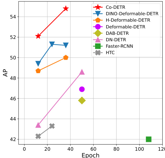
Figure 1. Performance of models with ResNet-50 on COCO val. $\mathcal{C}\mathrm{o}$ -DETR outperforms other counterparts by a large margin.
图 1: 使用 ResNet-50 的模型在 COCO val 上的性能。$\mathcal{C}\mathrm{o}$ -DETR 以显著优势超越其他对比模型。
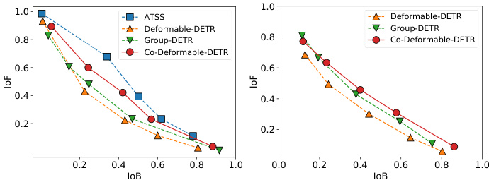
Figure 2. IoF-IoB curves for the feature disc rim inability score in the encoder and attention disc rim inability score in the decoder.
图 2: 编码器中特征判别力得分与解码器中注意力判别力得分的 IoF-IoB 曲线。
In this paper, we try to make DETR-based detectors superior to conventional detectors while maintaining their end-to-end merit. To address this challenge, we focus on the intuitive drawback of one-to-one set matching that it explores less positive queries. This will lead to severe inefficient training issues. We detailedly analyze this from two aspects, the latent representation generated by the encoder and the attention learning in the decoder. We first compare the disc rim inability score of the latent features between the Deformable-DETR [43] and the one-to-many label assignment method where we simply replace the decoder with the ATSS head. The feature $l^{2}$ -norm in each spatial coordinate is utilized to represent the disc rim inability score. Given the encoder’s output $\mathcal{F}\in\mathbb{R}^{C\times H\times W}$ , we can obtain the disc rim inability score map $S\in\mathbb{R}^{1\times H\times W}$ . The object can be better detected when the scores in the corresponding area are higher. As shown in Figure 2, we demonstrate the IoF-IoB curve (IoF: intersection over foreground, IoB: intersection over background) by applying different thresholds on the disc rim inability scores (details in Section 3.4). The higher IoF-IoB curve in ATSS indicates that it’s easier to distinguish the foreground and background. We further visualize the disc rim inability score map $s$ in Figure 3. It’s obvious that the features in some salient areas are fully activated in the one-to-many label assignment method but less explored in one-to-one set matching. For the exploration of decoder training, we also demonstrate the IoF-IoB curve of the cross-attention score in the decoder based on the Deformable-DETR and the Group-DETR [5] which introduces more positive queries into the decoder. The illustration in Figure 2 shows that too few positive queries also influence attention learning and increasing more positive queries in the decoder can slightly alleviate this.
本文致力于在保持端到端优势的同时,使基于DETR的检测器性能超越传统检测器。针对这一挑战,我们聚焦于一对一集合匹配的固有缺陷——正样本查询(positive queries)探索不足,这会导致严重的训练低效问题。我们从编码器生成的潜在表示和解码器的注意力学习两方面展开详细分析。
首先比较了Deformable-DETR [43]与一对多标签分配方法(仅将解码器替换为ATSS头)的潜在特征判别力得分。利用每个空间坐标中特征的$l^{2}$-范数表征判别力得分,给定编码器输出$\mathcal{F}\in\mathbb{R}^{C\times H\times W}$,可获得判别力得分图$S\in\mathbb{R}^{1\times H\times W}$。当对应区域得分越高时,目标检测效果越好。如图2所示,通过对判别力得分施加不同阈值(详见3.4节),我们绘制了IoF-IoB曲线(IoF:前景交并比,IoB:背景交并比)。ATSS中更高的IoF-IoB曲线表明其更易区分前景与背景。图3进一步可视化判别力得分图$s$,可见一对多方法能充分激活显著区域特征,而一对一集合匹配对此探索不足。
针对解码器训练分析,我们还基于Deformable-DETR和引入更多正样本查询的Group-DETR [5],绘制了解码器交叉注意力得分的IoF-IoB曲线。图2表明过少的正样本查询会影响注意力学习,而增加解码器中的正样本查询可略微缓解此问题。
This significant observation motivates us to present a simple but effective method, a collaborative hybrid assignment training scheme (Co-DETR). The key insight of $\mathcal{C}\mathrm{o}.$ - DETR is to use versatile one-to-many label assignments to improve the training efficiency and effectiveness of both the encoder and decoder. More specifically, we integrate the auxiliary heads with the output of the transformer encoder. These heads can be supervised by versatile one-to-many label assignments such as ATSS [41], FCOS [32], and Faster RCNN [27]. Different label assignments enrich the supervisions on the encoder’s output which forces it to be discri mi native enough to support the training convergence of these heads. To further improve the training efficiency of the decoder, we elaborately encode the coordinates of positive samples in these auxiliary heads, including the positive anchors and positive proposals. They are sent to the original decoder as multiple groups of positive queries to predict the pre-assigned categories and bounding boxes. Positive coordinates in each auxiliary head serve as an independent group that is isolated from the other groups. Versatile oneto-many label assignments can introduce lavish (positive query, ground-truth) pairs to improve the decoder’s training efficiency. Note that, only the original decoder is used during inference, thus the proposed training scheme only introduces extra overheads during training.
这一重要发现促使我们提出了一种简单而有效的方法——协作式混合分配训练方案 (Co-DETR)。Co-DETR 的核心思想是通过多样化的一对多标签分配 (one-to-many label assignments) 来提升编码器和解码器的训练效率与效果。具体而言,我们将辅助头 (auxiliary heads) 与 Transformer 编码器的输出进行集成。这些辅助头可以由 ATSS [41]、FCOS [32] 和 Faster RCNN [27] 等多种一对多标签分配方案进行监督。不同的标签分配方式丰富了编码器输出的监督信号,迫使其具备足够判别性以支持这些辅助头的训练收敛。为了进一步提升解码器的训练效率,我们精心编码了这些辅助头中正样本(包括正锚框和正提议框)的坐标信息,并将它们作为多组正查询 (positive queries) 输入原始解码器,用于预测预分配的类别和边界框。每个辅助头中的正样本坐标作为独立组别与其他组别隔离。多样化的一对多标签分配能够引入丰富的(正查询,真实标注)配对,从而提升解码器的训练效率。值得注意的是,推理阶段仅使用原始解码器,因此所提出的训练方案仅在训练时引入额外开销。
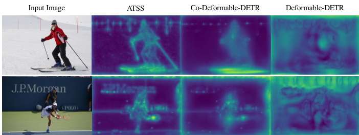
Figure 3. Visualization s of disc rim inability scores in the encoder.
图 3: 编码器中判别性得分的可视化。
We conduct extensive experiments to evaluate the efficiency and effectiveness of the proposed method. Illustrated in Figure 3, $\mathcal{C}\mathrm{o}$ -DETR greatly alleviates the poorly encoder’s feature learning in one-to-one set matching. As a plug-and-play approach, we easily combine it with different DETR variants, including DAB-DETR [23], DeformableDETR [43], and DINO-Deformable-DETR [39]. As shown in Figure 1, $\mathcal{C}\mathrm{o}$ -DETR achieves faster training convergence and even higher performance. Specifically, we improve the basic Deformable-DETR by $5.8%$ AP in 12-epoch training and $3.2%$ AP in 36-epoch training. The state-of-theart DINO-Deformable-DETR with Swin-L [25] can still be improved from $58.5%$ to $59.5%$ AP on COCO val. Surprisingly, incorporated with ViT-L [8] backbone, we achieve $66.0%$ AP on COCO test-dev and $67.9%$ AP on LVIS val, establishing the new state-of-the-art detector with much fewer model sizes.
我们进行了大量实验来评估所提方法的效率和效果。如图3所示,$\mathcal{C}\mathrm{o}$-DETR显著改善了一对一集合匹配中编码器特征学习不佳的问题。作为一种即插即用方案,我们轻松将其与多种DETR变体结合,包括DAB-DETR [23]、DeformableDETR [43]和DINO-Deformable-DETR [39]。如图1所示,$\mathcal{C}\mathrm{o}$-DETR实现了更快的训练收敛和更高性能。具体而言,我们将基础版Deformable-DETR在12轮训练中AP提升了5.8%,在36轮训练中AP提升了3.2%。采用Swin-L [25]的顶尖DINO-Deformable-DETR在COCO验证集上仍可从58.5% AP提升至59.5% AP。令人惊讶的是,结合ViT-L [8]骨干网络,我们在COCO测试集上达到66.0% AP,在LVIS验证集上达到67.9% AP,以更小的模型规模建立了新的检测器标杆。
2. Related Works
2. 相关工作
One-to-many label assignment. For one-to-many label assignment in object detection, multiple box candidates can be assigned to the same ground-truth box as positive samples in the training phase. In classic anchor-based detectors, such as Faster-RCNN [27] and RetinaNet [21], the sample selection is guided by the predefined IoU threshold and matching IoU between anchors and annotated boxes. The anchor-free FCOS [32] leverages the center priors and assigns spatial locations near the center of each bounding box as positives. Moreover, the adaptive mechanism is incorporated into one-to-many label assignments to overcome the limitation of fixed label assignments. ATSS [41] performs adaptive anchor selection by the statistical dynamic IoU values of top $k$ closest anchors. PAA [17] adaptively separates anchors into positive and negative samples in a probabilistic manner. In this paper, we propose a collaborative hybrid assignment scheme to improve encoder representations via auxiliary heads with one-to-many label assignments.
一对多标签分配。在目标检测的一对多标签分配中,训练阶段可以将多个候选框分配给同一个真实框作为正样本。经典基于锚点的检测器(如Faster-RCNN [27] 和 RetinaNet [21])通过预定义的IoU阈值以及锚点与标注框之间的匹配IoU来指导样本选择。无锚点检测器FCOS [32] 利用中心先验,将每个边界框中心附近的空间位置分配为正样本。此外,自适应机制被引入一对多标签分配以克服固定分配方式的局限性:ATSS [41] 通过统计前$k$个最近锚点的动态IoU值进行自适应锚点选择;PAA [17] 以概率方式自适应地将锚点划分为正负样本。本文提出协作式混合分配方案,通过配备一对多标签分配的辅助头来提升编码器表征能力。
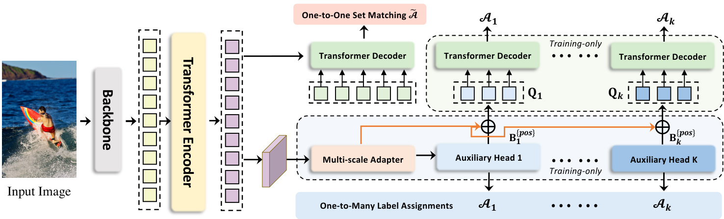
Figure 4. Framework of our Collaborative Hybrid Assignment Training. The auxiliary branches are discarded during evaluation.
图 4: 我们的协作混合分配训练框架。评估阶段会丢弃辅助分支。
One-to-one set matching. The pioneering transformerbased detector, DETR [1], incorporates the one-to-one set matching scheme into object detection and performs fully end-to-end object detection. The one-to-one set matching strategy first calculates the global matching cost via Hungarian matching and assigns only one positive sample with the minimum matching cost for each ground-truth box. DNDETR [18] demonstrates the slow convergence results from the instability of one-to-one set matching, thus introducing denoising training to eliminate this issue. DINO [39] inherits the advanced query formulation of DAB-DETR [23] and incorporates an improved contrastive denoising technique to achieve state-of-the-art performance. Group-DETR [5] constructs group-wise one-to-many label assignment to exploit multiple positive object queries, which is similar to the hybrid matching scheme in $\mathcal{H}$ -DETR [16]. In contrast with the above follow-up works, we present a new perspective of collaborative optimization for one-to-one set matching.
一对一集合匹配。开创性的基于Transformer的检测器DETR [1]将一对一集合匹配方案引入目标检测任务,实现了完全端到端的目标检测。该策略首先通过匈牙利匹配计算全局匹配代价,并为每个真实标注框仅分配一个具有最小匹配代价的正样本。DNDETR [18]揭示了因一对一集合匹配不稳定性导致的收敛缓慢问题,进而引入去噪训练来解决这一缺陷。DINO [39]继承了DAB-DETR [23]的高级查询构建方法,结合改进的对比去噪技术实现了最先进的性能。Group-DETR [5]构建了分组式一对多标签分配机制以利用多个正样本对象查询,其思路类似于$\mathcal{H}$-DETR [16]中的混合匹配方案。与上述后续研究不同,我们提出了一种针对一对一集合匹配的协同优化新视角。
3. Method
3. 方法
3.1. Overview
3.1. 概述
Following the standard DETR protocol, the input image is fed into the backbone and encoder to generate latent features. Multiple predefined object queries interact with them in the decoder via cross-attention afterwards. We introduce $\mathcal{C}\mathrm{o}$ -DETR to improve the feature learning in the encoder and the attention learning in the decoder via the collaborative hybrid assignments training scheme and the customized positive queries generation. We will detailedly describe these modules and give insights why they can work well.
遵循标准DETR协议,输入图像通过主干网络和编码器生成潜在特征。随后多个预定义物体查询(query)在解码器中通过交叉注意力机制与这些特征交互。我们提出的$\mathcal{C}\mathrm{o}$-DETR通过协作式混合分配训练方案和定制化正查询生成机制,改进了编码器的特征学习与解码器的注意力学习。下文将详细阐述这些模块并解析其有效性原理。
3.2. Collaborative Hybrid Assignments Training
3.2. 协作式混合分配训练
To alleviate the sparse supervision on the encoder’s output caused by the fewer positive queries in the decoder, we incorporate versatile auxiliary heads with different one-tomany label assignment paradigms, e.g., ATSS, and Faster R-CNN. Different label assignments enrich the supervisions on the encoder’s output which forces it to be discriminative enough to support the training convergence of these heads. Specifically, given the encoder’s latent feature $\mathcal{F}$ , we firstly transform it to the feature pyramid ${\mathcal{F}{1},\cdots,\mathcal{F}{J}}$ via the multi-scale adapter where $J$ indicates feature map with $2^{2+J}$ down sampling stride. Similar to ViTDet [20], the feature pyramid is constructed by a single feature map in the single-scale encoder, while we use bilinear interpolation and $3\times3$ convolution for upsampling. For instance, with the single-scale feature from the encoder, we successively apply down sampling $3\times3$ convolution with stride 2) or upsampling operations to produce a feature pyramid. As for the multi-scale encoder, we only downsample the coarsest feature in the multi-scale encoder features $\mathcal{F}$ to build the feature pyramid. Defined $K$ collaborative heads with corresponding label assignment manners $A_{k}$ , for the $i$ -th collaborative head, ${\mathcal{F}{1},\cdots,\mathcal{F}{J}}$ is sent to it to obtain the predictions $\hat{\mathbf{P}}{i}$ . At the $i$ -th head, $\mathcal{A}{i}$ is used to compute the supervised targets for the positive and negative samples in $\mathbf{P}_{i}$ . Denoted $\mathbf{G}$ as the ground-truth set, this procedure can be formulated as:
为缓解解码器中正样本查询较少导致编码器输出监督稀疏的问题,我们引入了采用不同一对多标签分配范式(如ATSS和Faster R-CNN)的多功能辅助头。不同的标签分配方式丰富了编码器输出的监督信号,迫使编码器具备足够判别性以支持这些辅助头的训练收敛。具体而言,给定编码器的潜在特征$\mathcal{F}$,我们首先通过多尺度适配器将其转换为特征金字塔${\mathcal{F}{1},\cdots,\mathcal{F}{J}}$,其中$J$表示下采样步长为$2^{2+J}$的特征图。与ViTDet [20]类似,该特征金字塔由单尺度编码器中的单一特征图构建,但我们采用双线性插值和$3\times3$卷积进行上采样。例如,对于编码器的单尺度特征,我们连续应用步长为2的$3\times3$下采样卷积或上采样操作来生成特征金字塔。对于多尺度编码器,我们仅对多尺度编码器特征$\mathcal{F}$中最粗糙的特征进行下采样以构建特征金字塔。定义$K$个具有相应标签分配方式$A{k}$的协作头,对于第$i$个协作头,将${\mathcal{F}{1},\cdots,\mathcal{F}{J}}$输入其中以获得预测结果$\hat{\mathbf{P}}{i}$。在第$i$个头中,$\mathcal{A}{i}$用于计算$\mathbf{P}_{i}$中正负样本的监督目标。设$\mathbf{G}$为真实标签集,该过程可表述为:
$$
\mathbf{P}{i}^{{p o s}},\mathbf{B}{i}^{{p o s}},\mathbf{P}{i}^{{n e g}}=\mathcal{A}{i}(\hat{\mathbf{P}}_{i},\mathbf{G}),
$$
$$
\mathbf{P}{i}^{{p o s}},\mathbf{B}{i}^{{p o s}},\mathbf{P}{i}^{{n e g}}=\mathcal{A}{i}(\hat{\mathbf{P}}_{i},\mathbf{G}),
$$
where ${p o s}$ and ${n e g}$ indicate the pair set of $(j$ , positive coordinates or negative coordinates in ${\mathcal{F}}{j}$ ) determined by $\mathcal{A}{i}$ . $j$ means the feature index in ${\mathcal{F}{1},\cdots,\mathcal{F}{J}}$ . $\mathbf{B}_{i}^{{p o s}}$ is the set of spatial positive coordinates. Pi{pos} and P{neg} are the supervised targets in the corresponding coordinates, including the categories and regressed offsets. To be specific, we describe the detailed information about each variable in Table 1. The loss functions can be defined as:
其中 ${pos}$ 和 ${neg}$ 表示由 $\mathcal{A}{i}$ 确定的 $(j$, ${\mathcal{F}}{j}$ 中正坐标或负坐标) 的配对集合。$j$ 表示 ${\mathcal{F}{1},\cdots,\mathcal{F}{J}}$ 中的特征索引。$\mathbf{B}{i}^{{pos}}$ 是空间正坐标的集合。$P_{i}^{{pos}}$ 和 $P^{{neg}}$ 是对应坐标中的监督目标,包括类别和回归偏移量。具体来说,我们在表1中描述了每个变量的详细信息。损失函数可以定义为:
Table 1. Detailed information of auxiliary heads. The auxiliary heads include Faster-RCNN [27], ATSS [41], RetinaNet [21], and FCOS [32]. If not otherwise specified, we follow the original implementations, e.g., anchor generation.
表 1: 辅助头部的详细信息。辅助头部包括 Faster-RCNN [27]、ATSS [41]、RetinaNet [21] 和 FCOS [32]。除非另有说明,否则我们遵循原始实现,例如锚点生成。
| Head i | Loss L | AssignmentA |
|---|---|---|
| Faster-RCNN [27] | cls:CE loss, reg: GIoU loss | {pos}: IoU(proposal, gt)>0.5 {neg}: IoU(proposal, gt)<0.5 |
| ATSS [41] | cls:Focal loss reg:GIoU, BCE loss | {pos}:IoU(anchor, gt)>(mean+std) {neg}:IoU(anchor,gt)<(mean+std) |
| RetinaNet [21] | cls:Focal loss reg:GIoU Loss | {pos}: IoU(anchor, gt)>0.5 {neg}: IoU(anchor, gt)<0.4 |
| FCOS [32] | cls:Focal Loss reg: GIoU, BCE loss | {pos}:points inside gt center area {neg}:points outside gt center area |
$$
\mathcal{L}{i}^{e n c}=\mathcal{L}{i}(\hat{\mathbf{P}}{i}^{{p o s}},\mathbf{P}{i}^{{p o s}})+\mathcal{L}{i}(\hat{\mathbf{P}}{i}^{{n e g}},\mathbf{P}_{i}^{{n e g}}),
$$
$$
\mathcal{L}{i}^{e n c}=\mathcal{L}{i}(\hat{\mathbf{P}}{i}^{{p o s}},\mathbf{P}{i}^{{p o s}})+\mathcal{L}{i}(\hat{\mathbf{P}}{i}^{{n e g}},\mathbf{P}_{i}^{{n e g}}),
$$
Note that the regression loss is discarded for negative samples. The training objective of the optimization for $K$ auxiliary heads is formulated as follows:
请注意,对于负样本会舍弃回归损失。针对 $K$ 个辅助头的优化训练目标定义如下:
$$
\mathcal{L}^{e n c}=\sum_{i=1}^{K}\mathcal{L}_{i}^{e n c}
$$
$$
\mathcal{L}^{e n c}=\sum_{i=1}^{K}\mathcal{L}_{i}^{e n c}
$$
3.3. Customized Positive Queries Generation
3.3. 定制化正向查询生成
In the one-to-one set matching paradigm, each groundtruth box will only be assigned to one specific query as the supervised target. Too few positive queries lead to inefficient cross-attention learning in the transformer decoder as shown in Figure 2. To alleviate this, we elaborately generate sufficient customized positive queries according to the label assignment $\mathcal{A}{i}$ in each auxiliary head. Specifically, given the positive coordinates set $\mathbf{B}{i}^{{p o s}}\in\mathbb{R}^{M_{i}\times4}$ in the $i\cdot$ -th auxiliary head, where $M_{i}$ is the number of positive samples, the extra customized positive queries $\bar{\mathbf{Q}}{i}\in\mathbb{R}^{M_{i}\times C}$ can be generated by:
在一对一集合匹配范式中,每个真实框只会被分配给一个特定查询作为监督目标。如图2所示,过少的正样本查询会导致Transformer解码器中的交叉注意力学习效率低下。为缓解这一问题,我们根据每个辅助头中的标签分配$\mathcal{A}{i}$精心生成足量的定制化正样本查询。具体而言,给定第$i$个辅助头中的正样本坐标集$\mathbf{B}{i}^{{pos}}\in\mathbb{R}^{M_{i}\times4}$(其中$M_{i}$为正样本数量),可通过以下方式生成额外的定制化正样本查询$\bar{\mathbf{Q}}{i}\in\mathbb{R}^{M_{i}\times C}$:
$$
\mathbf{Q}{i}=\operatorname{Linear}(\mathrm{PE}(\mathbf{B}{i}^{{p o s}}))+\operatorname{Linear}(\mathrm{E}({\mathcal{F}_{*}},{p o s})).
$$
$$
\mathbf{Q}{i}=\operatorname{Linear}(\mathrm{PE}(\mathbf{B}{i}^{{p o s}}))+\operatorname{Linear}(\mathrm{E}({\mathcal{F}_{*}},{p o s})).
$$
where $\mathrm{PE}(\cdot)$ stands for positional encodings and we select the corresponding features from $\operatorname{E}(\cdot)$ according to the index pair $j$ , positive coordinates or negative coordinates in ${\mathcal{F}}_{j}$ ).
其中 $\mathrm{PE}(\cdot)$ 表示位置编码 (positional encodings),我们根据索引对 $j$、正坐标或负坐标从 $\operatorname{E}(\cdot)$ 中选择 ${\mathcal{F}}_{j}$ 中对应的特征。
As a result, there are $K+1$ groups of queries that contribute to a single one-to-one set matching branch and $K$ branches with one-to-many label assignments during training. The auxiliary one-to-many label assignment branches share the same parameters with $L$ decoders layers in the original main branch. All the queries in the auxiliary branch are regarded as positive queries, thus the matching process is discarded. To be specific, the loss of the $l$ -th decoder layer in the $i$ -th auxiliary branch can be formulated as:
因此,在训练过程中,有 $K+1$ 组查询分别贡献于一个一对一集合匹配分支和 $K$ 个一对多标签分配分支。辅助的一对多标签分配分支与原始主分支中的 $L$ 个解码器层共享相同参数。辅助分支中的所有查询均被视为正样本查询,因此省略了匹配过程。具体而言,第 $i$ 个辅助分支中第 $l$ 个解码器层的损失可表示为:
$$
\mathcal{L}{i,l}^{d e c}=\widetilde{\mathcal{L}}(\widetilde{\mathbf{P}}{i,l},\mathbf{P}_{i}^{{p o s}}).
$$
$$
\mathcal{L}{i,l}^{d e c}=\widetilde{\mathcal{L}}(\widetilde{\mathbf{P}}{i,l},\mathbf{P}_{i}^{{p o s}}).
$$
$\widetilde{\mathbf{P}}_{i,l}$ refers to the output predictions of the $l$ -th decoder layer ien the $i$ -th auxiliary branch. Finally, the training objective for $\mathcal{C}\mathrm{o}$ -DETR is:
$\widetilde{\mathbf{P}}_{i,l}$ 表示第 $i$ 个辅助分支中第 $l$ 个解码器层的输出预测。最终,$\mathcal{C}\mathrm{o}$-DETR 的训练目标为:
$$
\mathcal{L}^{g l o b a l}=\sum_{l=1}^{L}(\widetilde{\mathcal{L}}{l}^{d e c}+\lambda_{1}\sum_{i=1}^{K}\mathcal{L}{i,l}^{d e c}+\lambda_{2}\mathcal{L}^{e n c}),
$$
$$
\mathcal{L}^{g l o b a l}=\sum_{l=1}^{L}(\widetilde{\mathcal{L}}{l}^{d e c}+\lambda_{1}\sum_{i=1}^{K}\mathcal{L}{i,l}^{d e c}+\lambda_{2}\mathcal{L}^{e n c}),
$$
where $\widetilde{\mathcal{L}}{l}^{d e c}$ stands for the loss in the original one-to-one set matchi neg branch [1], $\lambda_{1}$ and $\lambda_{2}$ are the coefficient balancing the losses.
其中 $\widetilde{\mathcal{L}}{l}^{d e c}$ 表示原始一对一集合匹配分支 [1] 中的损失,$\lambda_{1}$ 和 $\lambda_{2}$ 是用于平衡损失的系数。
3.4. Why Co-DETR works
3.4. 为什么Co-DETR有效
$\mathcal{C}\mathrm{o}$ -DETR leads to evident improvement to the DETRbased detectors. In the following, we try to investigate its effectiveness qualitatively and quantitatively. We conduct detailed analysis based on Deformable-DETR with ResNet50 [15] backbone using the 36-epoch setting.
$\mathcal{C}\mathrm{o}$ -DETR显著提升了基于DETR的检测器性能。下文我们将从定性和定量两个维度探究其有效性。实验采用ResNet50 [15] 主干网络和36训练周期的Deformable-DETR框架进行详细分析。
Enrich the encoder’s supervisions. Intuitively, too few positive queries lead to sparse supervisions as only one query is supervised by regression loss for each ground-truth. The positive samples in one-to-many label assignment manners receive more localization supervisions to help enhance the latent feature learning. To further explore how the sparse supervisions impede the model training, we detailedly investigate the latent features produced by the encoder. We introduce the IoF-IoB curve to quantize the disc rim in a bility score of the encoder’s output. Specifically, given the latent feature $\mathcal{F}$ of the encoder, inspired by the feature visualization in Figure 3, we compute the IoF (intersection over foreground) and IoB (intersection over background). Given the encoder’s feature $\mathcal{F}{j}\in\mathbb{R}^{C\times H{j}\times W_{j}}$ at level $j$ , we first calculate the $l^{2}$ -norm $\widehat{\mathcal{F}}{j}\in\mathbb{R}^{1\times H{j}\times W_{j}}$ and resize it to the image size $H\times W$ . bThe disc rim inability score $\mathcal{D}(\mathcal{F})$ is computed by averaging the scores from all levels:
增强编码器的监督信号。直观来看,过少的正样本查询会导致监督稀疏,因为每个真实标注仅通过回归损失监督一个查询。在一对多标签分配机制中,正样本能获得更多定位监督,从而促进潜在特征学习。为深入探究稀疏监督如何阻碍模型训练,我们详细分析了编码器生成的潜在特征。通过引入IoF-IoB曲线来量化编码器输出的边缘判别能力得分:给定编码器的潜在特征$\mathcal{F}$,受图3特征可视化的启发,我们计算前景交并比(IoF)与背景交并比(IoB)。对于第$j$层编码器特征$\mathcal{F}{j}\in\mathbb{R}^{C\times H{j}\times W_{j}}$,先计算其$l^{2}$范数$\widehat{\mathcal{F}}{j}\in\mathbb{R}^{1\times H{j}\times W_{j}}$并缩放到图像尺寸$H\times W$。边缘判别能力得分$\mathcal{D}(\mathcal{F})$通过对所有层级得分取平均得到:
$$
\mathcal{D}(\mathcal{F})=\frac{1}{J}\sum_{j=1}^{J}\frac{\widehat{\mathcal{F}}_{j}}{m a x(\widehat{\mathcal{F}}_{j})},
$$
$$
\mathcal{D}(\mathcal{F})=\frac{1}{J}\sum_{j=1}^{J}\frac{\widehat{\mathcal{F}}_{j}}{m a x(\widehat{\mathcal{F}}_{j})},
$$
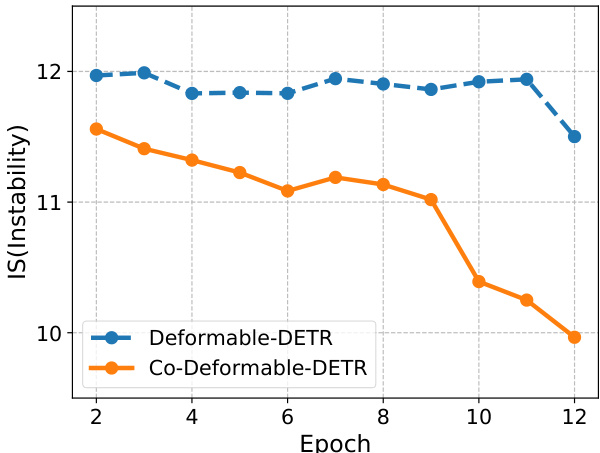
Figure 5. The instability (IS) [18] of Deformable-DETR and ${\mathcal{C}}_{0}.$ - Deformable-DETR on COCO dataset. These detectors are trained for 12 epochs with ResNet-50 backbones.
图 5: Deformable-DETR与${\mathcal{C}}_{0}$的不稳定性(IS) [18] - 基于COCO数据集使用ResNet-50骨干网络训练12个epoch的Deformable-DETR检测器。
where the resize operation is omitted. We visualize the disc rim inability scores of ATSS, Deformable-DETR, and our $\mathcal{C}\mathrm{o}$ -Deformable-DETR in Figure 3. Compared with Deformable-DETR, both ATSS and $\mathcal{C}\mathrm{o}$ -Deformable-DETR own stronger ability to distinguish the areas of key objects, while Deformable-DETR is almost disturbed by the background. Consequently, we define the indicators for foreground and background as $\mathbb{1}(D(\mathcal{F})>S)\in\mathbb{R}^{H\times W}$ and $\mathbb{1}(\mathcal{D}(\mathcal{F})<S)\in\mathbb{R}^{H\times W}$ , respectively. $S$ is a predefined score thresh, $\mathbb{1}(x)$ is 1 if $x$ is true and 0 otherwise. As for the mask of foreground Mfg ∈ RH×W , the element Mfh,gw is 1 if the point $(h,w)$ is inside the foreground and 0 otherwise. The area of intersection over foreground (IoF) $\mathcal{T}^{f g}$ can be computed as:
其中省略了调整大小的操作。我们在图3中可视化了ATSS、Deformable-DETR以及我们的$\mathcal{C}\mathrm{o}$-Deformable-DETR的圆盘边缘不可区分性分数。与Deformable-DETR相比,ATSS和$\mathcal{C}\mathrm{o}$-Deformable-DETR都具备更强的区分关键目标区域的能力,而Deformable-DETR几乎被背景干扰。因此,我们分别将前景和背景的指示器定义为$\mathbb{1}(D(\mathcal{F})>S)\in\mathbb{R}^{H\times W}$和$\mathbb{1}(\mathcal{D}(\mathcal{F})<S)\in\mathbb{R}^{H\times W}$。$S$是预定义的分数阈值,$\mathbb{1}(x)$在$x$为真时为1,否则为0。至于前景掩码Mfg ∈ RH×W,若点$(h,w)$位于前景内,则元素Mfh,gw为1,否则为0。前景交并比(IoF) $\mathcal{T}^{f g}$可计算为:
$$
\mathcal{T}^{f g}=\frac{\sum_{h=1}^{H}\sum_{w=1}^{W}(\mathbb{1}(\mathcal{D}(\mathcal{F}_{h,w})>S)\cdot\mathcal{M}_{h,w}^{f g})}{\sum_{h=1}^{H}\sum_{w=1}^{W}\mathcal{M}_{h,w}^{f g}}.
$$
$$
\mathcal{T}^{f g}=\frac{\sum_{h=1}^{H}\sum_{w=1}^{W}(\mathbb{1}(\mathcal{D}(\mathcal{F}_{h,w})>S)\cdot\mathcal{M}_{h,w}^{f g})}{\sum_{h=1}^{H}\sum_{w=1}^{W}\mathcal{M}_{h,w}^{f g}}.
$$
Concretely, we compute the area of intersection over background areas (IoB) in a similar way and plot the curve IoF and IoB by varying $S$ in Figure 2. Obviously, ATSS and $C\mathbf{0}$ -Deformable-DETR obtain higher IoF values than both Deformable-DETR and Group-DETR under the same IoB values, which demonstrates the encoder representations benefit from the one-to-many label assignment.
具体来说,我们以类似方式计算背景区域交并比(IoB),并通过调整$S$在图2中绘制IoF和IoB曲线。显然,在相同IoB值下,ATSS和$C\mathbf{0}$-Deformable-DETR获得的IoF值均高于Deformable-DETR和Group-DETR,这表明编码器表征受益于一对多标签分配策略。
Improve the cross-attention learning by reducing the instability of Hungarian matching. Hungarian matching is the core scheme in one-to-one set matching. Cross-attention is an important operation to help the positive queries encode abundant object information. It requires sufficient training to achieve this. We observe that the Hungarian matching introduces uncontrollable instability since the ground-truth assigned to a specific positive query in the same image is changing during the training process. Following [18], we present the comparison of instability in Figure 5, where we find our approach contributes to a more stable matching process. Furthermore, in order to quantify how well crossattention is being optimized, we also calculate the IoF-IoB curve for attention score. Similar to the feature discriminability score computation, we set different thresholds for attention score to get multiple IoF-IoB pairs. The comparisons between Deformable-DETR, Group-DETR, and CoDeformable-DETR can be viewed in Figure 2. We find that the IoF-IoB curves of DETRs with more positive queries are generally above Deformable-DETR, which is consistent with our motivation.
通过降低匈牙利匹配的不稳定性来改进交叉注意力学习。匈牙利匹配是一对一集合匹配的核心方案。交叉注意力是帮助正查询(positive queries)编码丰富目标信息的重要操作,需要充分训练才能实现。我们观察到匈牙利匹配会引入不可控的不稳定性,因为在训练过程中,同一图像中分配给特定正查询的真实标签(ground-truth)会不断变化。参照[18],我们在图5中展示了不稳定性对比,发现我们的方法能实现更稳定的匹配过程。此外,为量化交叉注意力的优化效果,我们还计算了注意力分数的IoF-IoB曲线。与特征可区分性得分的计算类似,我们为注意力分数设置不同阈值以获得多组IoF-IoB值。可变形DETR(Deformable-DETR)、分组DETR(Group-DETR)和协同可变形DETR(CoDeformable-DETR)的对比结果如图2所示。我们发现具有更多正查询的DETR模型,其IoF-IoB曲线通常位于可变形DETR上方,这与我们的设计动机一致。
3.5. Comparison with other methods
3.5. 与其他方法的对比
Differences between our method and other counterparts. Group-DETR, $\mathcal{H}$ -DETR, and SQR [2] perform oneto-many assignments by one-to-one matching with duplicate groups and repeated ground-truth boxes. $\mathcal{C}\mathrm{o}$ -DETR explicitly assigns multiple spatial coordinates as positives for each ground truth. Accordingly, these dense supervision signals are directly applied to the latent feature map to enable it more disc rim i native. By contrast, Group-DETR, $\mathcal{H}.$ - DETR, and SQR lack this mechanism. Although more positive queries are introduced in these counterparts, the oneto-many assignments implemented by Hungarian Matching still suffer from the instability issues of one-to-one matching. Our method benefits from the stability of off-theshelf one-to-many assignments and inherits their specific matching manner between positive queries and ground-truth boxes. Group-DETR and $\mathcal{H}$ -DETR fail to reveal the comple ment ari ties between one-to-one matching and traditional one-to-many assignment. To our best knowledge, we are the first to give the quantitative and qualitative analysis on the detectors with the traditional one-to-many assignment and one-to-one matching. This helps us better understand their differences and complement ari ties so that we can naturally improve the DETR’s learning ability by leveraging off-theshelf one-to-many assignment designs without requiring additional specialized one-to-many design experience.
我们的方法与其他方法的差异。Group-DETR、$\mathcal{H}$-DETR和SQR [2]通过单组重复和真实框复现的一对一匹配实现一对多分配。$\mathcal{C}\mathrm{o}$-DETR显式地为每个真实框分配多个空间坐标作为正样本,这些密集监督信号直接作用于潜在特征图以增强其判别性。相比之下,Group-DETR、$\mathcal{H}$-DETR和SQR缺乏这一机制。尽管这些方法引入了更多正样本查询(query),但基于匈牙利匹配实现的一对多分配仍受限于一对一匹配的不稳定性。我们的方法受益于现成一对多分配的稳定性,并继承了正样本查询与真实框间的特定匹配方式。Group-DETR和$\mathcal{H}$-DETR未能揭示一对一匹配与传统一对多分配的互补性。据我们所知,我们首次对传统一对多分配与一对一匹配的检测器进行了定量与定性分析,这有助于理解二者的差异与互补关系,从而无需额外专业设计经验即可自然提升DETR的学习能力。
No negative queries are introduced in the decoder. Duplicate object queries inevitably bring large amounts of negative queries for the decoder and a significant increase in GPU memory. However, our method only processes the positive coordinates in the decoder, thus consuming less memory as shown in Table 7.
解码器中没有引入负查询。重复的对象查询不可避免地会给解码器带来大量负查询,并显著增加GPU内存占用。然而,我们的方法仅处理解码器中的正坐标,因此内存消耗更低,如表7所示。
4. Experiments
4. 实验
4.1. Setup
4.1. 配置
Datasets and Evaluation Metrics. Our experiments are conducted on the MS COCO 2017 dataset [22] and LVIS v1.0 dataset [12]. The COCO dataset consists of 115K labeled images for training and 5K images for validation. We report the detection results by default on the val subset. The results of our largest model evaluated on the test-dev (20K images) are also reported. LVIS v1.0 is a large-scale and long-tail dataset with 1203 categories for large vocabulary instance segmentation. To verify the scalability of $\mathcal{C}\mathrm{o}$ -DETR, we further apply it to a large-scale object detection benchmark, namely Objects365 [30]. There are 1.7M labeled images used for training and 80K images for validation in the Objects365 dataset. All results follow the standard mean Average Precision(AP) under IoU thresholds ranging from 0.5 to 0.95 at different object scales.
数据集与评估指标。我们在MS COCO 2017数据集[22]和LVIS v1.0数据集[12]上进行实验。COCO数据集包含11.5万张训练图像和5000张验证图像,默认在验证集上报告检测结果,同时汇报最大模型在test-dev子集(2万张图像)上的评估结果。LVIS v1.0是一个包含1203个类别的大规模长尾分布数据集,用于大词汇量实例分割任务。为验证$\mathcal{C}\mathrm{o}$-DETR的扩展性,我们将其应用于Objects365[30]大规模目标检测基准,该数据集包含170万训练图像和8万验证图像。所有结果均采用标准平均精度均值(mAP)指标,在0.5至0.95交并比(IoU)阈值范围内评估不同尺度目标的性能。
| Method | K | #epochs | AP |
| Conditional DETR-C5[26] ConditionalDETR-C5 5[26] ConditionalDETR-C5 [26] DAB-DETR-C5 [23] | 0 1 2 0 | 36 36 36 36 | 39.4 41.5(+2.1) 41.8(+2.4) 41.2 |
| DAB-DETR-C5 [23] DAB-DETR-C5 [23] Deformable-DETR [43] Deformable-DETR[43] | 1 2 0 1 | 36 36 12 12 | 43.1(+1.9) 43.5(+2.3) 37.1 42.3(+5.2) |
| Deformable-DETR[43] Deformable-DETR [43] Deformable-DETR [43] | 0 1 2 | 12 36 36 36 | 42.9(+5.8) 43.3 46.8(+3.5) 46.5(+3.2) |
Table 2. Results of plain baselines on COCO val.
| 方法 | K | 训练轮数 | AP |
|---|---|---|---|
| Conditional DETR-C5 [26] | 0 | 36 | 39.4 |
| Conditional DETR-C5 [26] | 1 | 36 | 41.5 (+2.1) |
| Conditional DETR-C5 [26] | 2 | 36 | 41.8 (+2.4) |
| DAB-DETR-C5 [23] | 0 | 36 | 41.2 |
| DAB-DETR-C5 [23] | 1 | 36 | 43.1 (+1.9) |
| DAB-DETR-C5 [23] | 2 | 36 | 43.5 (+2.3) |
| Deformable-DETR [43] | 0 | 12 | 37.1 |
| Deformable-DETR [43] | 1 | 12 | 42.3 (+5.2) |
| Deformable-DETR [43] | 0 | 36 | 42.9 (+5.8) |
| Deformable-DETR [43] | 1 | 36 | 43.3 |
| Deformable-DETR [43] | 2 | 36 | 46.8 (+3.5) |
| Deformable-DETR [43] | 2 | 36 | 46.5 (+3.2) |
Implementation Details. We incorporate our $\mathcal{C}\mathrm{o}$ -DETR into the current DETR-like pipelines and keep the training setting consistent with the baselines. We adopt ATSS and Faster-RCNN as the auxiliary heads for $K=2$ and only keep ATSS for $K=1$ . More details about our auxiliary heads can be found in the supplementary materials. We choose the number of learnable object queries to 300 and set ${\lambda_{1},\lambda_{2}}$ to $\lbrace1.0,2.0\rbrace$ by default. For $\mathcal{C}\mathrm{o}$ -DINO- Deformable-DETR $^{++}$ , we use large-scale jitter with copypaste [10].
实现细节。我们将$\mathcal{C}\mathrm{o}$-DETR集成到当前类DETR流程中,并保持与基线一致的训练设置。对于$K=2$的情况采用ATSS和Faster-RCNN作为辅助头,$K=1$时仅保留ATSS。辅助头的更多细节详见补充材料。我们将可学习目标查询数量设为300,默认设置${\lambda_{1},\lambda_{2}}$为$\lbrace1.0,2.0\rbrace$。对于$\mathcal{C}\mathrm{o}$-DINO-Deformable-DETR$^{++}$,采用带copypaste[10]的大尺度抖动增强。
4.2. Main Results
4.2. 主要结果
In this section, we empirically analyze the effectiveness and generalization ability of $\mathcal{C}\mathrm{o}$ -DETR on different DETR variants in Table 2 and Table 3. All results are reproduced using mm detection [4]. We first apply the collaborative hybrid assignments training to single-scale DETRs with C5 features. Surprisingly, both Conditional-DETR and DAB-DETR obtain $2.4%$ and $2.3%$ AP gains over the baselines with a long training schedule. For DeformableDETR with multi-scale features, the detection performance is significantly boosted from $37.1%$ to $42.9%$ AP. The overall improvements $(+3.2%$ AP) still hold when the training time is increased to 36 epochs. Moreover, we conduct experiments on the improved Deformable-DETR (denoted as Deformable-DETR $^{++}$ ) following [16], where a $+2.4%$ AP gain is observed. The state-of-the-art DINO-Deformable
在本节中,我们通过实证分析$\mathcal{C}\mathrm{o}$-DETR在不同DETR变体上的有效性和泛化能力,结果如表2和表3所示。所有实验均使用mm detection [4]复现。我们首先将协同混合分配训练应用于具有C5特征的单尺度DETR。令人惊讶的是,Conditional-DETR和DAB-DETR在长训练周期下分别获得$2.4%$和$2.3%$的AP提升。对于具有多尺度特征的DeformableDETR,检测性能从$37.1%$显著提升至$42.9%$ AP。当训练周期延长至36轮时,整体改进$(+3.2%$ AP)仍然保持。此外,我们在改进版Deformable-DETR(记为Deformable-DETR$^{++}$)上按照[16]进行实验,观察到$+2.4%$ AP提升。当前最先进的DINO-Deformable
| Method | K | #epochs | AP |
| Deformable-DETR++[43] Deformable-DETR++[43] Deformable-DETR++[43] DINO-Deformable-DETR [39] | 0 1 2 0 | 12 12 12 | 47.1 48.7(+1.6) 49.5(+2.4) 49.4 |
| DINO-Deformable-DETRt [39] DINO-Deformable-DETRt [39] | 1 2 | 12 12 12 | 51.0(+1.6) 51.2(+1.8) |
| Deformable-DETR+++ [43] Deformable-DETR+++ [43] Deformable-DETR+++ [43] | 0 1 2 | 12 12 12 | 55.2 56.4(+1.2) 56.9(+1.7) |
| DINO-Deformable-DETR+ [39] DINO-Deformable-DETR+ [39] DINO-Deformable-DETR+ [39] | 0 1 2 | 12 12 12 | 58.5 59.3(+0.8) 59.5(+1.0) |
Table 3. Results of strong baselines on COCO val. Methods with $\dagger$ use 5 feature levels. $\ddagger$ refers to Swin-L backbone.
| 方法 | K | 训练轮数 | AP |
|---|---|---|---|
| Deformable-DETR++[43] Deformable-DETR++[43] Deformable-DETR++[43] DINO-Deformable-DETR [39] | 0 1 2 0 | 12 12 12 | 47.1 48.7(+1.6) 49.5(+2.4) 49.4 |
| DINO-Deformable-DETRt [39] DINO-Deformable-DETRt [39] | 1 2 | 12 12 12 | 51.0(+1.6) 51.2(+1.8) |
| Deformable-DETR+++ [43] Deformable-DETR+++ [43] Deformable-DETR+++ [43] | 0 1 2 | 12 12 12 | 55.2 56.4(+1.2) 56.9(+1.7) |
| DINO-Deformable-DETR+ [39] DINO-Deformable-DETR+ [39] DINO-Deformable-DETR+ [39] | 0 1 2 | 12 12 12 | 58.5 59.3(+0.8) 59.5(+1.0) |
表 3: COCO验证集上的强基线结果。带$\dagger$的方法使用5个特征层级,$\ddagger$表示采用Swin-L骨干网络。
DETR equipped with our method can achieve $51.2%$ AP, which is $+1.8%$ AP higher than the competitive baseline.
采用我们方法的DETR可实现51.2% AP (average precision) ,较竞争基线提升+1.8% AP。
We further scale up the backbone capacity from ResNet50 to Swin-L [25] based on two state-of-the-art baselines. As presented in Table 3, $\mathcal{C}\mathrm{o}$ -DETR achieves $56.9%$ AP and surpasses the Deformable $\mathrm{DETR++}$ baseline by a large margin $(+1.7%$ AP). The performance of DINODeformable-DETR with Swin-L can still be boosted from $58.5%$ to $59.5%$ AP.
我们基于两个最先进的基线模型,将骨干网络容量从ResNet50扩展到Swin-L [25]。如表3所示,Co-DETR实现了56.9%的平均精度(AP),大幅超越Deformable DETR++基线(+1.7% AP)。采用Swin-L的DINODeformable-DETR性能仍可从58.5%提升至59.5% AP。
4.3. Comparisons with the state-of-the-art
4.3. 与现有最优技术的比较
We apply our method with $K=2$ to Deformable $\mathrm{DETR++}$ and DINO. Besides, the quality focal loss [19] and NMS are adopted for our $\mathcal{C}\mathrm{o}$ -DINO-Deformable-DETR. We report the comparisons on COCO val in Table 4. Compared with other competitive counterparts, our method converges much faster. For example, $\mathcal{C}\mathrm{o}$ -DINO-DeformableDETR readily achieves $52.1%$ AP when using only 12 epochs with ResNet-50 backbone. Our method with SwinL can obtain $58.9%$ AP for $1\times$ scheduler, even surpassing other state-of-the-art frameworks on $3\times$ scheduler. More importantly, our best model $\mathcal{C}\mathrm{o}$ -DINO-Deformable $\mathrm{DETR++}$ achieves $54.8%$ AP with ResNet-50 and $60.7%$ AP with Swin-L under 36-epoch training, outperforming all existing detectors with the same backbone by clear margins.
我们将方法应用于 $K=2$ 的 Deformable $\mathrm{DETR++}$ 和 DINO。此外,我们的 $\mathcal{C}\mathrm{o}$-DINO-Deformable-DETR 采用了质量焦点损失 [19] 和非极大值抑制 (NMS)。表 4 展示了在 COCO val 上的对比结果。与其他竞争方法相比,我们的方法收敛速度显著更快。例如,$\mathcal{C}\mathrm{o}$-DINO-DeformableDETR 仅使用 12 个训练周期和 ResNet-50 骨干网络即可达到 $52.1%$ AP。采用 SwinL 骨干网络时,我们的方法在 $1\times$ 调度器下可获得 $58.9%$ AP,甚至超越了其他使用 $3\times$ 调度器的先进框架。更重要的是,我们的最佳模型 $\mathcal{C}\mathrm{o}$-DINO-Deformable $\mathrm{DETR++}$ 在 36 周期训练下,使用 ResNet-50 和 Swin-L 骨干网络分别达到 $54.8%$ 和 $60.7%$ AP,显著优于所有采用相同骨干网络的现有检测器。
To further explore the s cal ability of our method, we extend the backbone capacity to 304 million parameters. This large-scale backbone ViT-L [7] is pre-trained using a selfsupervised learning method (EVA-02 [8]). We first pre-train $\mathcal{C}\mathrm{o}$ -DINO-Deformable-DETR with ViT-L on Objects365 for 26 epochs, then fine-tune it on the COCO dataset for 12 epochs. In the fine-tuning stage, the input resolution is randomly selected between $480\times2400$ and $1536\times2400$ . The detailed settings are available in supplementary materials. Our results are evaluated with test-time augmentation. Table 5 presents the state-of-the-art comparisons on the
为了进一步探索我们方法的可扩展性,我们将骨干网络参数量扩展至3.04亿。这个大规模骨干网络ViT-L [7]采用自监督学习方法(EVA-02 [8])进行预训练。我们首先在Objects365数据集上用ViT-L预训练$\mathcal{C}\mathrm{o}$-DINO-Deformable-DETR 26个周期,然后在COCO数据集上微调12个周期。微调阶段输入分辨率在$480\times2400$和$1536\times2400$之间随机选择。详细设置见补充材料。我们的结果采用测试时增强进行评估。表5展示了当前最先进的
Table 4. Comparison to the state-of-the-art DETR variants on COCO val.
| Method | Backbone | Multi-scale | #query | #epochs | AP | AP50 | AP75 | APs | APM | APL |
| Conditional-DETR [26] | R50 | 300 | 108 | 43.0 | 64.0 | 45.7 | 22.7 | 46.7 | 61.5 | |
| Anchor-DETR [35] | R50 | 300 | 50 | 42.1 | 63.1 | 44.9 | 22.3 | 46.2 | 60.0 | |
| DAB-DETR [23] | R50 | 900 | 50 | 45.7 | 66.2 | 49.0 | 26.1 | 49.4 | 63.1 | |
| AdaMixer [9] | R50 | 300 | 36 | 47.0 | 66.0 | 51.1 | 30.1 | 50.2 | 61.8 | |
| Deformable-DETR [43] | R50 | 300 | 50 | 46.9 | 65.6 | 51.0 | 29.6 | 50.1 | 61.6 | |
| DN-Deformable-DETR [18] | R50 | 300 | 50 | 48.6 | 67.4 | 52.7 | 31.0 | 52.0 | 63.7 | |
| DINO-Deformable-DETR [39] | R50 | 900 | 12 | 49.4 | 66.9 | 53.8 | 32.3 | 52.5 | 63.9 | |
| DINO-Deformable-DETRt [39] | R50 | 900 | 36 | 51.2 | 69.0 | 55.8 | 35.0 | 54.3 | 65.3 | |
| DINO-Deformable-DETR [39] | Swin-L (IN-22K) | 900 | 36 | 58.5 | 77.0 | 64.1 | 41.5 | 62.3 | 74.0 | |
| Group-DINO-Deformable-DETR [5] | Swin-L (IN-22K) | 900 | 36 | 58.4 | 41.0 | 62.5 | 73.9 | |||
| H-Deformable-DETR [16] | R50 | 300 | 12 | 48.7 | 66.4 | 52.9 | 31.2 | 51.5 | 63.5 | |
| H-Deformable-DETR [16] | Swin-L (IN-22K) | 900 | 36 | 57.9 | 76.8 | 63.6 | 42.4 | 61.9 | 73.4 | |
| Co-Deformable-DETR | R50 | 300 | 12 | 49.5 | 67.6 | 54.3 | 32.4 | 52.7 | 63.7 | |
| Co-Deformable-DETR | Swin-L (IN-22K) | 900 | 36 | 58.5 | 77.1 | 64.5 | 42.4 | 62.4 | 74.0 | |
| Co-DINO-Deformable-DETRt | R50 | 900 | 12 | 52.1 | 69.4 | 57.1 | 35.4 | 55.4 | 65.9 | |
| Co-DINO-Deformable-DETRt | Swin-L (IN-22K) | 900 | 12 | 58.9 | 76.9 | 64.8 | 42.6 | 62.7 | 75.1 | |
| Co-DINO-Deformable-DETRt | Swin-L (IN-22K) | 900 | 24 | 59.8 | 77.7 | 65.5 | 43.6 | 63.5 | 75.5 | |
| Co-DINO-Deformable-DETRt | Swin-L (IN-22K) | 900 | 36 | 60.0 | 77.7 | 66.1 | 44.6 | 63.9 | 75.7 | |
| Co-DINO-Deformable-DETR++t | R50 | 900 | 12 | 52.1 | 69.3 | 57.3 | 35.4 | 55.5 | 67.2 | |
| Co-DINO-Deformable-DETR++t | R50 | 900 | 36 | 54.8 | 72.5 | 60.1 | 38.3 | 58.4 | 69.6 | |
| Co-DINO-Deformable-DETR++t | Swin-L (IN-22K) | 900 | 12 | 59.3 | 77.3 | 64.9 | 43.3 | 63.3 | 75.5 | |
| Co-DINO-Deformable-DETR++t | Swin-L (IN-22K) | 900 | 24 | 60.4 | 78.3 | 66.4 | 44.6 | 64.2 | 76.5 | |
| Co-DINO-Deformable-DETR++t | Swin-L (IN-22K) | 900 | 36 | 60.7 | 78.5 | 66.7 | 45.1 | 64.7 | 76.4 |
: 5 feature levels.
表 4: 在COCO验证集上与最先进DETR变体的对比
| 方法 | 主干网络 | 多尺度 | 查询数 | 训练轮数 | AP | AP50 | AP75 | APs | APM | APL |
|---|---|---|---|---|---|---|---|---|---|---|
| Conditional-DETR [26] | R50 | 300 | 108 | 43.0 | 64.0 | 45.7 | 22.7 | 46.7 | 61.5 | |
| Anchor-DETR [35] | R50 | 300 | 50 | 42.1 | 63.1 | 44.9 | 22.3 | 46.2 | 60.0 | |
| DAB-DETR [23] | R50 | 900 | 50 | 45.7 | 66.2 | 49.0 | 26.1 | 49.4 | 63.1 | |
| AdaMixer [9] | R50 | 300 | 36 | 47.0 | 66.0 | 51.1 | 30.1 | 50.2 | 61.8 | |
| Deformable-DETR [43] | R50 | 300 | 50 | 46.9 | 65.6 | 51.0 | 29.6 | 50.1 | 61.6 | |
| DN-Deformable-DETR [18] | R50 | 300 | 50 | 48.6 | 67.4 | 52.7 | 31.0 | 52.0 | 63.7 | |
| DINO-Deformable-DETR [39] | R50 | 900 | 12 | 49.4 | 66.9 | 53.8 | 32.3 | 52.5 | 63.9 | |
| DINO-Deformable-DETRt [39] | R50 | 900 | 36 | 51.2 | 69.0 | 55.8 | 35.0 | 54.3 | 65.3 | |
| DINO-Deformable-DETR [39] | Swin-L (IN-22K) | 900 | 36 | 58.5 | 77.0 | 64.1 | 41.5 | 62.3 | 74.0 | |
| Group-DINO-Deformable-DETR [5] | Swin-L (IN-22K) | 900 | 36 | 58.4 | 41.0 | 62.5 | 73.9 | |||
| H-Deformable-DETR [16] | R50 | 300 | 12 | 48.7 | 66.4 | 52.9 | 31.2 | 51.5 | 63.5 | |
| H-Deformable-DETR [16] | Swin-L (IN-22K) | 900 | 36 | 57.9 | 76.8 | 63.6 | 42.4 | 61.9 | 73.4 | |
| Co-Deformable-DETR | R50 | 300 | 12 | 49.5 | 67.6 | 54.3 | 32.4 | 52.7 | 63.7 | |
| Co-Deformable-DETR | Swin-L (IN-22K) | 900 | 36 | 58.5 | 77.1 | 64.5 | 42.4 | 62.4 | 74.0 | |
| Co-DINO-Deformable-DETRt | R50 | 900 | 12 | 52.1 | 69.4 | 57.1 | 35.4 | 55.4 | 65.9 | |
| Co-DINO-Deformable-DETRt | Swin-L (IN-22K) | 900 | 12 | 58.9 | 76.9 | 64.8 | 42.6 | 62.7 | 75.1 | |
| Co-DINO-Deformable-DETRt | Swin-L (IN-22K) | 900 | 24 | 59.8 | 77.7 | 65.5 | 43.6 | 63.5 | 75.5 | |
| Co-DINO-Deformable-DETRt | Swin-L (IN-22K) | 900 | 36 | 60.0 | 77.7 | 66.1 | 44.6 | 63.9 | 75.7 | |
| Co-DINO-Deformable-DETR++t | R50 | 900 | 12 | 52.1 | 69.3 | 57.3 | 35.4 | 55.5 | 67.2 | |
| Co-DINO-Deformable-DETR++t | R50 | 900 | 36 | 54.8 | 72.5 | 60.1 | 38.3 | 58.4 | 69.6 | |
| Co-DINO-Deformable-DETR++t | Swin-L (IN-22K) | 900 | 12 | 59.3 | 77.3 | 64.9 | 43.3 | 63.3 | 75.5 | |
| Co-DINO-Deformable-DETR++t | Swin-L (IN-22K) | 900 | 24 | 60.4 | 78.3 | 66.4 | 44.6 | 64.2 | 76.5 | |
| Co-DINO-Deformable-DETR++t | Swin-L (IN-22K) | 900 | 36 | 60.7 | 78.5 | 66.7 | 45.1 | 64.7 | 76.4 |
: 5个特征层级。
| Method | Backbone | enc. #params | val Apbor | test-dev Apbor |
| HTC++ [3] | SwinV2-G[24] | 3.0B | 62.5 | 63.1 |
| DINO [39] | Swin-L [25] | 218M | 63.2 | 63.3 |
| BEIT3 [33] | ViT-g [7] | 1.9B | 63.7 | |
| FD [36] | SwinV2-G [24] | 3.0B | 64.2 | |
| DINO [39] | FocalNet-H[38] | 746M | 64.2 | 64.3 |
| Group DETRv2 [6] | ViT-H [7] | 629M | 64.5 | |
| EVA-02 [8] | ViT-L [7] | 304M | 64.1 | 64.5 |
| DINO [39] | InternImage-G [34] | 3.0B | 65.3 | 65.5 |
| Co-DETR | ViT-L [7] | 304M | 65.9 | 66.0 |
Table 5. Comparison to the state-of-the-art frameworks on COCO.
| 方法 | 主干网络 | 编码器参数量 | 验证集 Apbor | 测试集 Apbor |
|---|---|---|---|---|
| HTC++ [3] | SwinV2-G [24] | 3.0B | 62.5 | 63.1 |
| DINO [39] | Swin-L [25] | 218M | 63.2 | 63.3 |
| BEIT3 [33] | ViT-g [7] | 1.9B | 63.7 | |
| FD [36] | SwinV2-G [24] | 3.0B | 64.2 | |
| DINO [39] | FocalNet-H [38] | 746M | 64.2 | 64.3 |
| Group DETRv2 [6] | ViT-H [7] | 629M | 64.5 | |
| EVA-02 [8] | ViT-L [7] | 304M | 64.1 | 64.5 |
| DINO [39] | InternImage-G [34] | 3.0B | 65.3 | 65.5 |
| Co-DETR | ViT-L [7] | 304M | 65.9 | 66.0 |
表 5. COCO数据集上先进框架的对比结果
COCO test-dev benchmark. With much fewer model sizes (304M parameters), $\mathcal{C}\mathrm{o}$ -DETR sets a new record of $66.0%$ AP on COCO test-dev, outperforming the previous best model Intern Image-G [34] by $+0.5%$ AP.
COCO test-dev基准测试。在模型参数量大幅减少(仅3.04亿参数)的情况下,$\mathcal{C}\mathrm{o}$-DETR以66.0% AP的成绩刷新了COCO test-dev纪录,较此前最佳模型Intern Image-G [34]提升了+0.5% AP。
We also demonstrate the best results of $\mathcal{C}\mathrm{{o}}$ -DETR on the long-tailed LVIS detection dataset. In particular, we use the same $\mathcal{C}\mathrm{o}$ -DINO-Deformable-DETR $^{++}$ as the model on COCO but choose FedLoss [42] as the classification loss to remedy the impact of unbalanced data distribution. Here, we only apply bounding boxes supervision and report the object detection results. The comparisons are available in Table 6. $\mathcal{C}\mathrm{o}$ -DETR with Swin-L yields $56.9%$ and $62.3%$ AP on LVIS val and minival, surpassing ViTDet with MAE-pretrained [13] ViT-H and GLIPv2 [40] by $+3.5%$ and $+2.5%$ AP, respectively. We further finetune the Objects365 pretrained $\mathcal{C}\mathrm{o}$ -DETR on this dataset. Without elaborate test-time augmentation, our approach achieves the best detection performance of $67.9%$ and $71.9%$ AP on LVIS val and minival. Compared to the 3-billion parameter Intern Image-G with test-time augmentation, we obtain $+4.7%$ and $+6.1%$ AP gains on LVIS val and minival while reducing the model size to 1/10.
我们还展示了 $\mathcal{C}\mathrm{{o}}$ -DETR 在长尾 LVIS 检测数据集上的最佳结果。具体而言,我们使用与 COCO 相同的 $\mathcal{C}\mathrm{o}$ -DINO-Deformable-DETR$^{++}$ 模型,但选择 FedLoss [42] 作为分类损失以缓解数据分布不平衡的影响。此处仅应用边界框监督并报告目标检测结果。对比结果如表 6 所示。采用 Swin-L 的 $\mathcal{C}\mathrm{o}$ -DETR 在 LVIS val 和 minival 上分别达到 $56.9%$ 和 $62.3%$ AP,较 MAE 预训练 [13] ViT-H 的 ViTDet 和 GLIPv2 [40] 分别提升 $+3.5%$ 和 $+2.5%$ AP。我们进一步在该数据集上微调了 Objects365 预训练的 $\mathcal{C}\mathrm{o}$ -DETR。无需复杂的测试时增强,我们的方法在 LVIS val 和 minival 上实现了 $67.9%$ 和 $71.9%$ AP 的最佳检测性能。相比采用测试时增强的 30 亿参数 Intern Image-G,我们在 LVIS val 和 minival 上分别获得 $+4.7%$ 和 $+6.1%$ AP 提升,同时将模型尺寸缩减至 1/10。
| Method | Backbone | enc. #params | val Apbor | minival Apboc |
| H-DETR [16] | Swin-L [25] | 218M | 47.9 | |
| ViTDet [20] | ViT-L [7] | 307M | 51.2 | |
| ViTDet [20] | ViT-H [7] | 632M | 53.4 | 1 |
| GLIPv2 [40] | Swin-H [25] | 637M | 1 | 59.8 |
| DINO [39] | InternImage-G [34] | 3.0B | 63.2 | 65.8 |
| EVA-02 [8] | ViT-L [7] | 304M | 65.2 | |
| Co-DETR | Swin-L [25] | 218M | 56.9 | - |
| Co-DETR | ViT-L [7] | 304M | 67.9 | 62.3 71.9 |
Table 6. Comparison to the state-of-the-art frameworks on LVIS.
| 方法 | 主干网络 | 编码器参数量 | val Apbor | minival Apboc |
|---|---|---|---|---|
| H-DETR [16] | Swin-L [25] | 218M | 47.9 | |
| ViTDet [20] | ViT-L [7] | 307M | 51.2 | |
| ViTDet [20] | ViT-H [7] | 632M | 53.4 | 1 |
| GLIPv2 [40] | Swin-H [25] | 637M | 1 | 59.8 |
| DINO [39] | InternImage-G [34] | 3.0B | 63.2 | 65.8 |
| EVA-02 [8] | ViT-L [7] | 304M | 65.2 | |
| Co-DETR | Swin-L [25] | 218M | 56.9 | - |
| Co-DETR | ViT-L [7] | 304M | 67.9 | 62.3 71.9 |
表 6. LVIS数据集上先进框架的对比结果
4.4. Ablation Studies
4.4. 消融实验
Unless stated otherwise, all experiments for ablations are conducted on Deformable-DETR with a ResNet-50 backbone. We choose the number of auxiliary heads $K$ to 1 by default and set the total batch size to 32. More ablations and analyses can be found in the supplementary materials.
除非另有说明,所有消融实验均在基于ResNet-50骨干网络的Deformable-DETR上进行。默认设置辅助头数量$K$为1,总批次大小设为32。更多消融实验与分析结果可查阅补充材料。
Table 7. Experimental results of $K$ varying from 1 to 6.
| Method | K | Auxiliary | Memory (MB) | GPU hours | AP |
| head | 12808 | 70 | |||
| Deformable-DETR++ | 0 | 15307 | 104 | 47.1 48.4 | |
| H-Deformable-DETR | 0 | ATSS | 13947 | 86 | 48.7 |
| Deformable-DETR++ Deformable-DETR++ | 2 | ATSS+PAA | 14629 | 124 | 49.0 |
| Deformable-DETR++ | 2 | ATSS+Faster-RCNN | 14387 | 120 | 49.5 |
| Deformable-DETR++ | 3 | ATSS+Faster-RCNN | 15263 | 150 | 49.5 |
| Deformable-DETR++ | 6 | + PAA ATSS+Faster-RCNN +PAA+RetinaNet +FCOS+GFL | 19385 | 280 | 48.9 |
表 7. $K$ 从1到6变化的实验结果。
| 方法 | K | 辅助头 | 内存 (MB) | GPU小时 | AP |
|---|---|---|---|---|---|
| Deformable-DETR++ | 0 | 15307 | 104 | 47.1 48.4 | |
| H-Deformable-DETR | 0 | ATSS | 13947 | 86 | 48.7 |
| Deformable-DETR++ Deformable-DETR++ | 2 | ATSS+PAA | 14629 | 124 | 49.0 |
| Deformable-DETR++ | 2 | ATSS+Faster-RCNN | 14387 | 120 | 49.5 |
| Deformable-DETR++ | 3 | ATSS+Faster-RCNN | 15263 | 150 | 49.5 |
| Deformable-DETR++ | 6 | + PAA ATSS+Faster-RCNN +PAA+RetinaNet +FCOS+GFL | 19385 | 280 | 48.9 |
| Auxiliary head | #epochs | AP | AP50 | AP75 |
| Baseline | 36 | 43.3 | 62.3 | 47.1 |
| RetinaNet [21] Faster-RCNN [27] | 36 36 | 46.1 46.3 | 64.2 64.7 | 50.1 50.5 |
| Mask-RCNN [14] | 36 | 46.5 | 65.0 | 50.6 |
| FCOS [32] | 36 | 46.5 | 64.8 | 50.7 |
| PAA [17] | 36 | 46.5 | 64.6 | 50.7 |
| GFL [19] ATSS [41] | 36 36 | 46.5 46.8 | 65.0 65.1 | 51.0 51.5 |
Table 8. Performance of our approach with various auxiliary oneto-many heads on COCO val.
| 辅助头 (Auxiliary head) | 训练轮数 (#epochs) | AP | AP50 | AP75 |
|---|---|---|---|---|
| 基线 (Baseline) | 36 | 43.3 | 62.3 | 47.1 |
| RetinaNet [21] Faster-RCNN [27] | 36 36 | 46.1 46.3 | 64.2 64.7 | 50.1 50.5 |
| Mask-RCNN [14] | 36 | 46.5 | 65.0 | 50.6 |
| FCOS [32] | 36 | 46.5 | 64.8 | 50.7 |
| PAA [17] | 36 | 46.5 | 64.6 | 50.7 |
| GFL [19] ATSS [41] | 36 36 | 46.5 46.8 | 65.0 65.1 | 51.0 51.5 |
表 8: 我们的方法在COCO验证集上使用不同辅助一对多头 (auxiliary one-to-many heads) 的性能表现。
Criteria for choosing auxiliary heads. We further delve into the criteria for choosing auxiliary heads in Table 7 and 8. The results in Table 8 reveal that any auxiliary head with one-to-many label assignments consistently improves the baseline and ATSS achieves the best performance. We find the accuracy continues to increase as $K$ increases when choosing $K$ smaller than 3. It is worth noting that performance degradation occurs when $K=6$ , and we speculate the severe conflicts among auxiliary heads cause this. If the feature learning is inconsistent across the auxiliary heads, the continuous improvement as $K$ becomes larger will be destroyed. We also analyze the optimization consistency of multiple heads next and in the supplementary materials. In summary, we can choose any head as the auxiliary head and we regard ATSS and Faster-RCNN as the common practice to achieve the best performance when $K\leq2$ . We do not use too many different heads, e.g., 6 different heads to avoid optimization conflicts.
选择辅助头的标准。我们进一步在表7和表8中探讨了选择辅助头的标准。表8的结果表明,任何具有一对多标签分配的辅助头都能持续提升基线性能,其中ATSS取得了最佳表现。我们发现当 $K$ 小于3时,准确率随着 $K$ 的增加而持续提升。值得注意的是,当 $K=6$ 时会出现性能下降,我们推测这是由于辅助头之间严重的冲突导致的。如果各辅助头的特征学习不一致,随着 $K$ 增大带来的持续改进就会被破坏。我们接下来及补充材料中还会分析多头优化的稳定性。综上所述,我们可以选择任意头作为辅助头,并建议在 $K\leq2$ 时采用ATSS和Faster-RCNN作为最佳实践方案。为避免优化冲突,我们不会使用过多不同头(例如6个不同头)。
Conflicts analysis. The conflicts emerge when the same spatial coordinate is assigned to different foreground boxes or treated as background in different auxiliary heads and can confuse the training of the detector. We first define the distance between head $H_{i}$ and head $H_{j}$ , and the average distance of $H_{i}$ to measure the optimization conflicts as:
冲突分析。当同一空间坐标被分配给不同的前景框或在不同的辅助头中被视为背景时,就会产生冲突,这可能会干扰检测器的训练。我们首先定义头 $H_{i}$ 和头 $H_{j}$ 之间的距离,以及 $H_{i}$ 的平均距离,以衡量优化冲突:
$$
S_{i,j}=\frac{1}{|\mathbf{D}|}\sum_{\mathbf{I}\in\mathbf{D}}\mathrm{KL}(\mathcal{C}(H_{i}(\mathbf{I})),\mathcal{C}(H_{j}(\mathbf{I})),
$$
$$
S_{i,j}=\frac{1}{|\mathbf{D}|}\sum_{\mathbf{I}\in\mathbf{D}}\mathrm{KL}(\mathcal{C}(H_{i}(\mathbf{I})),\mathcal{C}(H_{j}(\mathbf{I})),
$$

Figure 6. The distance when varying $K$ from 1 to 6.
图 6: 当 $K$ 从 1 变化到 6 时的距离。
| aux head | pos queries | #epochs | AP | AP50 | AP75 |
| 12 36 | 37.1 43.3 | 55.5 62.3 | 40.0 47.1 | ||
| √ | 12 36 | 41.6(+4.5) 46.2(+2.9) | 59.8 64.7 | 45.6 50.9 | |
| 12 36 | 40.5(+3.4) 45.3(+2.0) | 58.8 63.5 | 44.4 49.8 | ||
| 12 36 | 42.3(+5.2) 46.8(+3.5) | 60.5 65.1 | 46.1 51.5 |
Table 9. “aux head” denotes training with an auxiliary head and “pos queries” means the customized positive queries generation.
| aux head | pos queries | #epochs | AP | AP50 | AP75 |
|---|---|---|---|---|---|
| 12 36 | 37.1 43.3 | 55.5 62.3 | 40.0 47.1 | ||
| √ | 12 36 | 41.6(+4.5) 46.2(+2.9) | 59.8 64.7 | 45.6 50.9 | |
| 12 36 | 40.5(+3.4) 45.3(+2.0) | 58.8 63.5 | 44.4 49.8 | ||
| 12 36 | 42.3(+5.2) 46.8(+3.5) | 60.5 65.1 | 46.1 51.5 |
表 9: "aux head"表示使用辅助头训练,"pos queries"表示定制化的正查询生成。
$$
S_{i}=\frac{1}{2(K-1)}\sum_{j\neq i}^{K}(S_{i,j}+S_{j,i}),
$$
$$
S_{i}=\frac{1}{2(K-1)}\sum_{j\neq i}^{K}(S_{i,j}+S_{j,i}),
$$
where KL, D, I, $\mathcal{C}$ refer to KL divergence, dataset, the input image, and class activation maps (CAM) [29]. As illustrated in Figure 6, we compute the average distances among auxiliary heads for $K>1$ and the distance between the DETR head and the single auxiliary head for $K=1$ . We find the distance metric is insignificant for each auxiliary head when $K=1$ and this observation is consistent with our results in Table 8: the DETR head can be collaborative ly improved with any head when $K=1$ . When $K$ is increased to 2, the distance metrics increase slightly and our method achieves the best performance as shown in Table 7. The distance surges when $K$ is increased from 3 and 6, indicating severe optimization conflicts among these auxiliary heads lead to a decrease in performance. However, the baseline with 6 ATSS achieves $49.5%$ AP and can be decreased to $48.9%$ AP by replacing ATSS with 6 various heads. Accordingly, we speculate too many diverse auxiliary heads, e.g., more than 3 different heads, exacerbate the conflicts. In summary, optimization conflicts are influenced by the number of various auxiliary heads and the relations among these heads.
其中KL、D、I、$\mathcal{C}$分别指KL散度、数据集、输入图像和类别激活图(CAM) [29]。如图6所示,我们计算了$K>1$时各辅助头之间的平均距离,以及$K=1$时DETR头与单个辅助头之间的距离。发现当$K=1$时,各辅助头的距离度量并不显著,这一观察结果与表8中的数据一致:当$K=1$时,DETR头可与任意辅助头协同提升。当$K$增至2时,距离度量略有上升,此时我们的方法取得了最佳性能(见表7)。当$K$从3增至6时距离急剧攀升,表明这些辅助头间严重的优化冲突导致了性能下降。不过,使用6个ATSS头的基线模型获得49.5% AP,而替换为6个不同头后AP降至48.9%。由此我们推测,过多差异性辅助头(如超过3种不同类型)会加剧冲突。综上,优化冲突受辅助头数量及其相互关系的影响。
Should the added heads be different? Collaborative training with two ATSS heads $(49.2%$ AP) still improves the model with one ATSS head $48.7%$ AP) as ATSS is complementary to the DETR head in our analysis. Besides, introducing a diverse and complementary auxiliary head rather than the same one as the original head, e.g., Faster-RCNN, can bring better gains $(49.5%$ AP). Note that this is not contradictory to above conclusion; instead, we can obtain the best performance with few different heads $\zeta\leq2,$ as the conflicts are insignificant, but we are faced with severe conflicts when using many different heads $\mathit{\check{K}}>3,$ ).
新增头部是否需要不同?双ATSS头部协同训练 $(49.2%$ AP) 仍优于单ATSS头部模型 $(48.7%$ AP),因ATSS头部与DETR头部在本分析中具有互补性。此外,引入多样化且互补的辅助头部(如Faster-RCNN)而非与原头部相同的结构,可获得更大提升 $(49.5%$ AP)。需注意这与前文结论并不矛盾:当使用少量差异化头部时 $\zeta\leq2,$ 冲突较小可获得最佳性能;而采用过多差异化头部 $\mathit{\check{K}}>3,$ 则会导致严重冲突。
Table 10. Comparison to baselines with longer schedule.
| Method | K | #epochs | GPUhours | AP |
| Deformable-DETR | 1 | 36 | 288 | 46.8 |
| Deformable-DETR | 0 | 50 | 333 | 44.5 |
| Deformable-DETR | 0 | 100 | 667 | 46.0 |
| Deformable-DETR | 0 | 150 | 1000 | 45.9 |
表 10: 与更长训练计划的基线对比
| 方法 | K | 训练轮数 | GPU小时数 | AP |
|---|---|---|---|---|
| Deformable-DETR | 1 | 36 | 288 | 46.8 |
| Deformable-DETR | 0 | 50 | 333 | 44.5 |
| Deformable-DETR | 0 | 100 | 667 | 46.0 |
| Deformable-DETR | 0 | 150 | 1000 | 45.9 |
| Branch | NMS | K = 0 | K = 1 | K=2 |
| Deformable-DETR++ | 47.1 | 48.7(+1.6) | 49.5(+2.4) | |
| ATSS | √ | 46.8 | 47.4(+0.6) | 48.0(+1.2) |
| Faster-RCNN | 45.9 | 46.7(+0.8) |
Table 11. Collaborative training consistently improves performances of all branches on Deformable-DETR $^{++}$ with ResNet-50.
| 分支 | NMS | K = 0 | K = 1 | K = 2 |
|---|---|---|---|---|
| Deformable-DETR++ | 47.1 | 48.7 (+1.6) | 49.5 (+2.4) | |
| ATSS | √ | 46.8 | 47.4 (+0.6) | 48.0 (+1.2) |
| Faster-RCNN | 45.9 | 46.7 (+0.8) |
表 11. 协同训练持续提升所有分支在 ResNet-50 架构的 Deformable-DETR$^{++}$上的性能表现。
The effect of each component. We perform a componentwise ablation to thoroughly analyze the effect of each component in Table 9. Incorporating the auxiliary head yields significant gains since the dense spatial supervision enables the encoder features more disc rim i native. Alternatively, introducing customized positive queries also contributes remarkably to the final results, while improving the training efficiency of the one-to-one set matching. Both techniques can accelerate convergence and improve performance. In summary, we observe the overall improvements stem from more disc rim i native features for the encoder and more efficient attention learning for the decoder.
各组件的作用分析。我们在表9中进行了逐组件消融实验以全面分析各模块的影响。引入辅助头 (auxiliary head) 带来显著提升,因为密集空间监督使编码器特征更具判别性 (discriminative)。此外,定制化正查询 (customized positive queries) 的引入也对最终结果产生显著贡献,同时提升了一对一集合匹配的训练效率。这两项技术都能加速收敛并提升性能。总体而言,我们发现改进主要源于编码器更具判别性的特征和解码器更高效的注意力学习。
Comparisons to the longer training schedule. As presented in Table 10, we find Deformable-DETR can not benefit from longer training as the performance saturates. On the contrary, $\mathcal{C}\mathrm{o}$ -DETR greatly accelerates the convergence as well as increasing the peak performance.
与更长训练周期的对比。如表 10 所示,我们发现 Deformable-DETR 无法从更长训练中受益,因为性能已趋于饱和。相反,$\mathcal{C}\mathrm{o}$-DETR 显著加快了收敛速度并提升了峰值性能。
Performance of auxiliary branches. Surprisingly, we observe $\mathcal{C}\mathrm{o}$ -DETR also brings consistent gains for auxiliary heads in Table 11. This implies our training paradigm contributes to more disc rim i native encoder representations, which improves the performances of both decoder and auxiliary heads.
辅助分支性能。令人惊讶的是,我们在表11中观察到 $\mathcal{C}\mathrm{o}$ -DETR 也为辅助头带来了持续增益。这表明我们的训练范式有助于生成更具判别性的编码器表征 (encoder representations) ,从而同时提升解码器和辅助头的性能。
Difference in distribution of original and customized positive queries. We visualize the positions of original positive queries and customized positive queries in Figure 7a. We only show one object (green box) per image. Positive queries assigned by Hungarian Matching in the decoder are marked in red. We mark positive queries extracted from Faster-RCNN and ATSS in blue and orange, respectively. These customized queries are distributed around the center region of the instance and provide sufficient supervision signals for the detector.
原始与定制化正查询的分布差异。我们在图7a中可视化原始正查询和定制化正查询的位置,每张图像仅显示一个目标(绿色框)。解码器中通过匈牙利匹配分配的正查询标记为红色,从Faster-RCNN和ATSS提取的正查询分别用蓝色和橙色标记。这些定制化查询分布在实例中心区域周围,为检测器提供了充分的监督信号。

Figure 7. Distribution of original and customized queries.
图 7: 原始查询与定制化查询的分布情况。
Does distribution difference lead to instability? We compute the average distance between original and customized queries in Figure 7b. The average distance between original negative queries and customized positive queries is significantly larger than the distance between original and customized positive queries. As this distribution gap between original and customized queries is marginal, there is no instability encountered during training.
分布差异会导致不稳定性吗?我们在图7b中计算了原始查询与定制查询之间的平均距离。原始负面查询与定制正面查询之间的平均距离显著大于原始与定制正面查询之间的距离。由于原始查询与定制查询之间的分布差距较小,训练过程中未出现不稳定性。
5. Conclusions
5. 结论
In this paper, we present a novel collaborative hybrid assignments training scheme, namely $\mathcal{C}\mathrm{o}$ -DETR, to learn more efficient and effective DETR-based detectors from versatile label assignment manners. This new training scheme can easily enhance the encoder’s learning ability in end-to-end detectors by training the multiple parallel auxiliary heads supervised by one-to-many label assignments. In addition, we conduct extra customized positive queries by extracting the positive coordinates from these auxiliary heads to improve the training efficiency of positive samples in decoder. Extensive experiments on COCO dataset demonstrate the efficiency and effectiveness of ${\mathcal{C}}_{0}.$ - DETR. Surprisingly, incorporated with ViT-L backbone, we achieve $66.0%$ AP on COCO test-dev and $67.9%$ AP on LVIS val, establishing the new state-of-the-art detector with much fewer model sizes.
本文提出了一种新颖的协同混合分配训练方案 $\mathcal{C}\mathrm{o}$ -DETR,旨在通过多样化标签分配方式学习更高效、更有效的基于DETR的检测器。该训练方案通过在一对多标签分配监督下训练多个并行辅助头,可显著增强端到端检测器中编码器的学习能力。此外,我们通过从这些辅助头提取正样本坐标来构建定制化正查询,从而提升解码器中正样本的训练效率。在COCO数据集上的大量实验验证了 ${\mathcal{C}}_{0}.$ -DETR的高效性。值得注意的是,结合ViT-L主干网络时,我们在COCO test-dev上达到66.0% AP,在LVIS val上达到67.9% AP,以更小的模型尺寸建立了全新最优检测器。
References
参考文献
DETRs with Collaborative Hybrid Assignments Training
基于协作混合分配训练的DETR模型
Supplementary Material
补充材料
Table 12. Influence of number of convolutions in auxiliary head.
| #convs | 0 | 1 | 2 | 3 | 4 | 5 |
| AP | 41.8 | 42.3 | 41.9 | 42.1 | 42.3 | 42.0 |
表 12: 辅助头中卷积次数的影响
| #convs | 0 | 1 | 2 | 3 | 4 | 5 |
|---|---|---|---|---|---|---|
| AP | 41.8 | 42.3 | 41.9 | 42.1 | 42.3 | 42.0 |
Table 13. Results of hyper-parameter tuning for $\lambda_{1}$ and $\lambda_{2}$ .
| 入1 | 入2 | #epochs | AP | APs | APM | APL |
| 0.25 0.5 1.0 2.0 | 2.0 2.0 2.0 2.0 | 36 36 36 36 | 46.2 46.6 46.8 46.1 | 28.3 29.0 28.1 27.4 | 49.7 50.5 50.6 49.7 | 60.4 61.2 61.3 61.4 |
| 1.0 1.0 1.0 | 1.0 2.0 3.0 | 36 36 36 | 46.1 46.8 46.5 | 27.9 28.1 29.3 | 49.7 50.6 50.4 | 60.9 61.3 61.4 61.0 |
表 13. 超参数 $\lambda_{1}$ 和 $\lambda_{2}$ 的调优结果
| λ1 | λ2 | #epochs | AP | APs | APM | APL |
|---|---|---|---|---|---|---|
| 0.25 0.5 1.0 2.0 | 2.0 2.0 2.0 2.0 | 36 36 36 36 | 46.2 46.6 46.8 46.1 | 28.3 29.0 28.1 27.4 | 49.7 50.5 50.6 49.7 | 60.4 61.2 61.3 61.4 |
| 1.0 1.0 1.0 | 1.0 2.0 3.0 | 36 36 36 | 46.1 46.8 46.5 | 27.9 28.1 29.3 | 49.7 50.6 50.4 | 60.9 61.3 61.4 61.0 |

Figure 8. The relation matrix for the DETR head, ATSS head, and Faster-RCNN head. The detector is $\mathcal{C}\mathrm{o}$ -Deformable-DETR $K=2$ ) with ResNet-50.
图 8: DETR头、ATSS头和Faster-RCNN头的关系矩阵。检测器为$\mathcal{C}\mathrm{o}$-Deformable-DETR ($K=2$)搭配ResNet-50。
A. More ablation studies
A. 更多消融实验
The number of stacked convolutions. Table 12 reveals our method is robust for the number of stacked convolutions in the auxiliary head (trained for 12 epochs). Concretely, we simply choose only 1 shared convolution to enable lightweight while achieving higher performance.
堆叠卷积层数。表12显示我们的方法对辅助头(训练12个周期)中的堆叠卷积层数具有鲁棒性。具体而言,我们仅选择1个共享卷积层来实现轻量化,同时获得更高性能。
Loss weights of collaborative training. Experimental results related to weighting the coefficient $\lambda_{1}$ and $\lambda_{2}$ are presented in Table 13. We find the proposed method is quite insensitive to the variations of ${\lambda_{1},\lambda_{2}}$ , since the performance slightly fluctuates when varying the loss coefficients. In summary, the coefficients ${\lambda_{1},\lambda_{2}}$ are robust and we set ${\lambda_{1},\lambda_{2}}$ to $\lbrace1.0,2.0\rbrace$ by default.
协作训练的损失权重。与系数$\lambda_{1}$和$\lambda_{2}$权重相关的实验结果如表13所示。我们发现该方法对${\lambda_{1},\lambda_{2}}$的变化相当不敏感,因为性能在损失系数变化时仅有轻微波动。综上所述,系数${\lambda_{1},\lambda_{2}}$具有鲁棒性,默认情况下我们将其设置为$\lbrace1.0,2.0\rbrace$。

Figure 9. Distances among 7 various heads in our model with $K=6$ .
图 9: 我们模型中 $K=6$ 时7个不同注意力头之间的距离。
The number of customized positive queries. We compute the average ratio of positive samples in one-to-many label assignment to the ground-truth boxes. For instance, the ratio is 18.7 for Faster-RCNN and 8.8 for ATSS on COCO dataset, indicating more than $8\times$ extra positive queries are introduced when $K=1$ .
自定义正样本查询数量。我们计算了一对多标签分配中正样本与真实标注框的平均比例。例如,在COCO数据集上,Faster-RCNN的比例为18.7,ATSS为8.8,这表明当$K=1$时引入了超过$8\times$的额外正样本查询。
Effectiveness of collaborative one-to-many label assignments. To verify the effectiveness of our feature learning mechanism, we compare our approach with Group-DETR (3 groups) and $\mathcal{H}$ -DETR. First, we find $\mathcal{C}\mathrm{o}$ -DETR performs better than hybrid matching scheme [16] while training faster and requiring less GPU memory in Table 6. As shown in Table 8, our method $K=1$ ) achieves $46.2%$ AP, surpassing Group-DETR ( $44.6%$ AP) by a large margin even without the customized positive queries generation. More importantly, the IoF-IoB curve in Figure 2 demonstrates Group-DETR fails to enhance the feature representations in the encoder, while our method alleviates the poorly feature learning.
协作式一对多标签分配的有效性。为验证我们特征学习机制的有效性,我们将本方法与Group-DETR(3组)和$\mathcal{H}$-DETR进行对比。首先如表6所示,$\mathcal{C}\mathrm{o}$-DETR在训练速度更快、GPU内存占用更低的同时,性能优于混合匹配方案[16]。如表8所示,我们的方法($K=1$)取得了$46.2%$AP,即使不使用定制化正查询生成,仍大幅超越Group-DETR($44.6%$AP)。更重要的是,图2中的IoF-IoB曲线表明Group-DETR未能增强编码器的特征表示,而我们的方法缓解了特征学习不足的问题。
Conflicts analysis. We have defined the distance between head $H_{i}$ and head $H_{j}$ , and the average distance of $H_{i}$ to measure the optimization conflicts in this study:
冲突分析。我们定义了头 $H_{i}$ 与头 $H_{j}$ 之间的距离,以及 $H_{i}$ 的平均距离来衡量本研究中的优化冲突:
$$
\mathcal{S}{i,j}=\frac{1}{|\mathbf{D}|}\sum_{\mathbf{I}\in\mathbf{D}}\mathrm{KL}(\mathcal{C}(H_{i}(\mathbf{I})),\mathcal{C}(H_{j}(\mathbf{I})),
$$
$$
\mathcal{S}{i,j}=\frac{1}{|\mathbf{D}|}\sum_{\mathbf{I}\in\mathbf{D}}\mathrm{KL}(\mathcal{C}(H_{i}(\mathbf{I})),\mathcal{C}(H_{j}(\mathbf{I})),
$$
$$
S_{i}=\frac{1}{2(K-1)}\sum_{j\neq i}^{K}(S_{i,j}+S_{j,i}),
$$
$$
S_{i}=\frac{1}{2(K-1)}\sum_{j\neq i}^{K}(S_{i,j}+S_{j,i}),
$$
where KL, D, I, $\mathcal{C}$ refer to KL divergence, dataset, the input image, and class activation maps (CAM) [29]. In our implementation, we choose the validation set COCO val as $\mathbf{D}$ and Grad-CAM as $\mathcal{C}$ . We use the output features of DETR encoder to compute the CAM maps. More specifically, we show the detailed distances when $K=2$ and $K=6$ in Figure 8 and Figure 9, res pet iv ely. The larger distance metric of $S_{i,j}$ indicates $H_{i}$ is less consistent to $H_{j}$ and contributes to the optimization inconsistency.
其中KL、D、I、$\mathcal{C}$分别指KL散度(KL divergence)、数据集(dataset)、输入图像(input image)和类别激活图(class activation maps, CAM) [29]。在实现中,我们选择COCO验证集(COCO val)作为$\mathbf{D}$,并采用Grad-CAM作为$\mathcal{C}$。我们使用DETR编码器的输出特征来计算CAM图。具体而言,图8和图9分别展示了$K=2$和$K=6$时的详细距离值。$S_{i,j}$的距离度量值越大,表明$H_{i}$与$H_{j}$的一致性越低,从而导致优化不一致性。
B. More implementation details
B. 更多实现细节
One-stage auxiliary heads. Based on the conventional one-stage detectors, we experiment with various first-stage designs [17, 19, 21, 32, 41] for the auxiliary heads. First, we use the GIoU [28] loss for the one-stage heads. Then, the number of stacked convolutions is reduced from 4 to 1. Such modification improves the training efficiency without any accuracy drop. For anchor-free detectors, e.g., FCOS [32], we assign the width of $8\times2^{j}$ and height of $8\times2^{j}$ for the positive coordinates with stride $2^{j}$ .
单阶段辅助头。基于传统单阶段检测器,我们对辅助头的多种第一阶段设计[17,19,21,32,41]进行了实验。首先,我们对单阶段头使用GIoU[28]损失函数。随后,将堆叠卷积层数从4层减少到1层。这种改进在不损失精度的前提下提升了训练效率。对于无锚检测器(如FCOS[32]),我们为步长为$2^{j}$的正坐标分配宽度$8\times2^{j}$和高度$8\times2^{j}$。
Two-stage auxiliary heads. We adopt the RPN and RCNN as our two-stage auxiliary heads based on the popular Faster-RCNN [27] and Mask-RCNN [14] detectors. To make $\mathcal{C}\mathrm{o}$ -DETR compatible with various detection heads, we adopt the same multi-scale features (stride 8 to stride 128) as the one-stage paradigm for two-stage auxiliary heads. Moreover, we adopt the GIoU loss for regression in the RCNN stage.
两阶段辅助头。我们基于流行的Faster-RCNN [27]和Mask-RCNN [14]检测器,采用RPN和RCNN作为两阶段辅助头。为使$\mathcal{C}\mathrm{o}$-DETR兼容各类检测头,我们对两阶段辅助头采用与单阶段范式相同的多尺度特征(步长8至步长128)。此外,在RCNN阶段采用GIoU损失进行回归。
System-level comparison on COCO. We first initialize the ViT-L backbone with EVA-02 weights. Then we perform intermediate finetuning on the Objects365 dataset using $\mathcal{C}\mathrm{o}$ -DINO-Deformable-DETR for 26 epochs and reduce the learning rate by a factor of 0.1 at epoch 24. The initial learning rate is $2.5\times10^{-4}$ and the batch size is 224. We choose the maximum size of input images as 1280 and randomly resize the shorter size to 480−1024. Moreover, we use 1500 object queries and $1000~\mathrm{DN}$ queries for this model. Finally, we finetune $\mathcal{C}\mathrm{o}$ -DETR on COCO for 12 epochs with an initial learning rate of $5\times10^{-5}$ and drop the learning rate at the 8-th epoch by multiplying 0.1. The shorter size of input images is enlarged to 480−1536 and the longer size is no more than 2400. We employ EMA and train this model with a batch size of 64.
COCO数据集上的系统级对比。我们首先使用EVA-02权重初始化ViT-L骨干网络,随后在Objects365数据集上采用$\mathcal{C}\mathrm{o}$-DINO-Deformable-DETR进行26轮中间微调,并在第24轮时将学习率降至0.1倍。初始学习率为$2.5\times10^{-4}$,批量大小为224。输入图像的最大尺寸设为1280,较短边随机缩放至480−1024范围。该模型采用1500个目标查询和$1000~\mathrm{DN}$查询。最后,我们在COCO数据集上用$\mathcal{C}\mathrm{o}$-DETR进行12轮微调,初始学习率为$5\times10^{-5}$,并在第8轮时以0.1倍率衰减学习率。输入图像的较短边扩大至480−1536,较长边不超过2400。采用EMA策略,以64的批量大小训练该模型。
System-level comparison on LVIS. In contrast to the COCO setting, we use $\mathcal{C}\mathrm{o}$ -DINO-Deformable $\mathrm{{DETR++}}$ to perform intermediate finetuning on the Objects365 dataset, as we find LSJ augmentation works better on the LVIS dataset. A batch size of 192, an initial learning rate of $2\times10^{-4}$ , and an input image size of $1280\times1280$ are used. We use 900 object queries and $1000\mathrm{DN}$ queries for this model. During finetuning on LVIS, we arm it with an additional auxiliary mask branch and increase the input size to $1536\times1536$ . Besides, we train the model without EMA for
LVIS上的系统级对比。与COCO设置不同,我们使用$\mathcal{C}\mathrm{o}$-DINO-Deformable $\mathrm{{DETR++}}$在Objects365数据集上进行中间微调,因为我们发现LSJ增强在LVIS数据集上效果更好。采用192的批次大小、$2\times10^{-4}$的初始学习率和$1280\times1280$的输入图像尺寸。该模型使用900个目标查询和$1000\mathrm{DN}$查询。在LVIS微调阶段,我们为其添加了额外的辅助掩码分支,并将输入尺寸提升至$1536\times1536$。此外,模型训练时未采用EMA(指数移动平均)。
16 epochs, where the batch size is set to 64, and the initial learning rate is set to $5\times10^{-5}$ , which is reduced by a factor of 0.1 at the 9-th and 15-th epoch.
16个周期,其中批次大小设置为64,初始学习率设为$5\times10^{-5}$,并在第9和第15周期时降低为原来的0.1倍。