一种零样本/少样本异常分类与分割方法:CVPR 2023 VAND研讨会挑战赛赛道1&2夺冠(零样本异常检测第1名,少样本异常检测第4名)
Abstract
摘要
In this technical report, we briefly introduce our solution for the Zero/Few-shot Track of the Visual Anomaly and Novelty Detection (VAND) 2023 Challenge. For industrial vi- sual inspection, building a single model that can be rapidly adapted to numerous categories without or with only a few normal reference images is a promising research direction. This is primarily because of the vast variety of the product types. For the zero-shot track, we propose a solution based on the CLIP model by adding extra linear layers. These layers are used to map the image features to the joint embedding space, so that they can compare with the text features to generate the anomaly maps. Besides, when the reference images are available, we utilize multiple memory banks to store their features and compare them with the features of the test images during the testing phase. In this challenge, our method achieved first place in the zero-shot track, especially excelling in segmentation with an impressive F1 score improvement of 0.0489 over the second-ranked participant. Furthermore, in the few-shot track, we secured the fourth position overall, with our classification F1 score of 0.8687 ranking first among all participating teams1.
在本技术报告中,我们简要介绍了针对2023年视觉异常与新颖性检测(VAND)挑战赛零样本/少样本赛道的解决方案。对于工业视觉检测而言,构建一个无需或仅需少量正常参考图像就能快速适配众多品类的单一模型,是一个极具前景的研究方向。这主要源于产品类型的极端多样性。
在零样本赛道中,我们提出了一种基于CLIP模型的解决方案,通过添加额外的线性层将图像特征映射到联合嵌入空间,使其能够与文本特征进行比较以生成异常热力图。此外,当参考图像可用时,我们利用多个记忆库存储其特征,并在测试阶段与测试图像特征进行比对。
本次挑战赛中,我们的方法在零样本赛道获得第一名,尤其在分割任务中以0.0489的F1分数优势显著领先第二名。在少样本赛道中,我们综合排名第四,其中分类F1分数0.8687在所有参赛团队中位列榜首[1]。
1. Introduction
1. 引言
In the field of computer vision, unsupervised anomaly detection (AD) [5, 9, 14, 16, 17] aims to identify abnormal images and locate anomalous regions using a model trained solely on anomaly-free images. It is widely used in industrial defect detection [1, 2, 12]. Most previous methods have centered on training dedicated models for each category, relying on a vast collection of normal images as references [15, 18]. In real-world applications, however, there are a wide variety of industrial products to be detected, and it is difficult to collect a large number of training images for each category. As a result, the zero/few-shot setting plays a crucial role in bringing AD to practical applications.
在计算机视觉领域,无监督异常检测 (AD) [5, 9, 14, 16, 17] 旨在仅使用正常图像训练的模型来识别异常图像并定位异常区域。该方法被广泛应用于工业缺陷检测 [1, 2, 12]。以往大多数方法都专注于为每个类别训练专用模型,依赖大量正常图像作为参考 [15, 18]。然而在实际应用中,待检测的工业产品种类繁多,难以收集每个类别的大量训练图像。因此,零样本/少样本设置对于推动异常检测走向实际应用至关重要。
WinCLIP [8], built on the open-source vision-language model CLIP [3, 13], is a model that can be rapidly adapted to abundant categories without or with only a handful of normal images. It assumes that language is able to aid zero/few-shot AD and proposes a window-based strategy to perform segmentation. Taking inspiration from it, we also followed the pattern of language guided AD and employed CLIP as our baseline.
WinCLIP [8]基于开源视觉语言模型CLIP [3, 13],是一种无需或仅需少量正常图像即可快速适配海量类别的模型。该研究假设语言能够辅助零样本/少样本异常检测 (AD),并提出基于窗口的分割策略。受此启发,我们同样遵循语言引导的异常检测范式,并采用CLIP作为基线模型。
Specifically, we adhere to the overall framework of CLIP for zero-shot classification and employ a combination of state and template ensembles to craft our text prompts. In order to locate the abnormal regions, we introduce extra linear layers to map the image features extracted from the CLIP image encoder to the linear space where the text features are located. Then, we make similarity comparison between the mapped image features and the text features, so as to obtain the corresponding anomaly maps. For the fewshot case, we retain the extra linear layers of the zero-shot phase and maintain their weights. In addition, we use the image encoder to extract the features of the reference images and save them to the memory bank for comparison with the features of the test images during the test phase. Note that, to fully take advantage of the shallow and deep features, we leverage features from different stages for both the zero and few shot settings.
具体而言,我们遵循CLIP的零样本分类整体框架,采用状态和模板组合的方式来构建文本提示。为了定位异常区域,我们引入了额外的线性层,将CLIP图像编码器提取的图像特征映射到文本特征所在的线性空间。然后,我们对映射后的图像特征和文本特征进行相似性比较,从而获得相应的异常图。对于少样本情况,我们保留了零样本阶段的额外线性层并保持其权重不变。此外,我们使用图像编码器提取参考图像的特征,并将其保存到记忆库中,以便在测试阶段与测试图像的特征进行比较。值得注意的是,为了充分利用浅层和深层特征,我们在零样本和少样本设置中都利用了来自不同阶段的特征。
Our method demonstrates strong competitiveness in both zero-shot and few-shot anomaly classification and segmentation. In the zero-shot track of the VAND Challenge, we achieve the first rank, surpassing the second-ranked approach by 0.0633 in overall score and 0.0489 in segmentation F1 score. In the few-shot track, we rank fourth overall, but our classification F1 score of 0.8687 places us first, surpassing the second-ranked approach by 0.0207.
我们的方法在零样本和少样本异常分类与分割任务中均展现出强劲竞争力。在VAND挑战赛的零样本赛道中,我们以总分0.0633和分割F1分数0.0489的优势超越第二名,获得榜首。在少样本赛道中,我们综合排名第四,但0.8687的分类F1分数位列第一,领先第二名0.0207。
2. Methodology
2. 方法论
Our approach is based on the CLIP [13] model, an opensource vision-language model that inherently possesses the capability for zero-shot classification. This implies that CLIP may be directly applicable to zero-shot anomaly classification. Furthermore, we made slight modifications to this model to enable its usage in anomaly segmentation and extended its applicability to the few-shot domain.
我们的方法基于CLIP [13]模型,这是一个开源的视觉语言模型,天生具备零样本分类能力。这意味着CLIP可能直接适用于零样本异常分类。此外,我们对该模型进行了轻微修改,使其能够用于异常分割,并将其适用性扩展到少样本领域。
2.1. Zero-shot AD Setting
2.1. 零样本 (Zero-shot) AD 设置
Anomaly Classification. We employ a binary zero-shot anomaly classification framework proposed by [8], which necessitates descriptions for both normal and abnormal objects. We further improve the detection accuracy by utilizing a text prompt ensemble strategy, including both state and template-level. For the state-level, we adapt generic text to describe the normal and abnormal objects (e.g., flawless, damaged), rather than providing excessively detailed descriptions such as “chip around edge and corner”. For the template-level, we screen the 85 templates in CLIP for ImageNet [6] and remove some templates that are not suitable for AD, such as “a photo of the weird [obj.]”.
异常分类。我们采用[8]提出的二元零样本异常分类框架,该框架需要正常和异常对象的描述。通过使用文本提示集成策略(包括状态级和模板级),我们进一步提高了检测精度。在状态级,我们调整通用文本来描述正常和异常对象(如无瑕疵、损坏),而不是提供过于详细的描述,例如"边缘和角落有缺口"。在模板级,我们从CLIP for ImageNet [6]的85个模板中筛选,并移除一些不适合异常检测的模板,例如"一张奇怪的[obj.]照片"。
We combine templates with the states of objects and mean the text features extracted by the text encoder as the final text features $F_{t}\in\mathbb{R}^{2\times C}$ , where C represents the number of channels of the feature. Let $F_{c}\in\mathbb{R}^{1\times C}$ represent the image features used for classification, and the relative probabilities $s$ of the object image being classified as normal or abnormal can be represented as,
我们将模板与对象状态结合,并将文本编码器提取的文本特征作为最终文本特征 $F_{t}\in\mathbb{R}^{2\times C}$ ,其中C表示特征的通道数。设 $F_{c}\in\mathbb{R}^{1\times C}$ 表示用于分类的图像特征,对象图像被分类为正常或异常的相对概率 $s$ 可表示为,
$$
{\boldsymbol{s}}=\operatorname{softmax}({\boldsymbol{F_{c}}}{\boldsymbol{F_{t}}}^{T}),
$$
$$
{\boldsymbol{s}}=\operatorname{softmax}({\boldsymbol{F_{c}}}{\boldsymbol{F_{t}}}^{T}),
$$
we use the probability corresponding to the anomaly as the anomaly score for the image.
我们使用异常对应的概率作为图像的异常分数。
Anomaly Segmentation. The structure of the image encoder of CLIP model can be based on either transformer or CNN. Although not used in the classification task, both archi tec ture s are capable of extracting features that preserve spacial information. These features can be represented as $\bar{F_{s}^{n}}\in\mathbb{R}^{H\times W\times C_{s}}$ , where $n$ indicates that the features are extracted by the $n$ -th stage in the image encoder.
异常分割。CLIP模型的图像编码器结构可基于Transformer或CNN架构。虽然在分类任务中未被使用,但两种架构都能提取保留空间信息的特征。这些特征可表示为$\bar{F_{s}^{n}}\in\mathbb{R}^{H\times W\times C_{s}}$,其中$n$表示特征由图像编码器第$n$阶段提取。
It is a natural idea to obtain the anomaly maps by calculating the similarity between the image features $F_{s}^{n}$ and the text features. However, since the CLIP model is designed for classification, image features other than those used for classification are not mapped to the joint embedding space. That is, these features cannot be compared directly to the text features in that space. As a result, we propose to map these image features into the joint embedding space by adding an additional linear layer, and then compare them with the text features.
通过计算图像特征 $F_{s}^{n}$ 与文本特征之间的相似性来获取异常图是一种自然的思路。然而,由于 CLIP 模型是为分类任务设计的,除分类用途外的图像特征并未映射到联合嵌入空间。也就是说,这些特征无法直接在该空间中与文本特征进行比较。因此,我们提出通过添加额外的线性层将这些图像特征映射到联合嵌入空间,再与文本特征进行对比。
In addition, we leverage the distinct features offered by the shallow and deep layers of the image encoder. The whole process is represented in the blue dashed box in Fig. 1. Taking the transformer based architecture ViT [7] as an example, we empirically divide all layers into four stages and use a linear layer for each stage to map the output features into the joint embedding space,
此外,我们利用图像编码器浅层和深层提供的不同特征。整个过程如图1中的蓝色虚线框所示。以基于Transformer架构的ViT [7]为例,我们实证将所有层划分为四个阶段,并为每个阶段使用一个线性层将输出特征映射到联合嵌入空间。
$$
F_{s}^{n\prime}=k^{n}F_{s}^{n}+b^{n},
$$
$$
F_{s}^{n\prime}=k^{n}F_{s}^{n}+b^{n},
$$
where $F_{s}^{n}$ here refers to the features of the patch tokens, and $k^{n}$ and $b^{n}$ represent weights and bias of the corresponding linear layer respectively. To obtain the anomaly maps for different stages, we make similarity comparison between the adjusted features $F_{s}^{n\prime}\in\mathbb{R}^{H W\times C}$ and the text features $F_{t}$ stage by stage. The final anomaly map $\mathbf{M}$ can be obtained by adding up the results for all the stages,
其中 $F_{s}^{n}$ 表示图像块(patch) token的特征,$k^{n}$ 和 $b^{n}$ 分别代表对应线性层的权重和偏置。为获取不同阶段的异常图,我们逐级比较调整后的特征 $F_{s}^{n\prime}\in\mathbb{R}^{H W\times C}$ 与文本特征 $F_{t}$ 的相似度。最终异常图 $\mathbf{M}$ 可通过累加所有阶段的结果获得。
$$
\mathbf{M}=\sum_{n}\operatorname{softmax}(F_{s}^{n^{\prime}}F_{t}^{\phantom{\dagger}T}).
$$
$$
\mathbf{M}=\sum_{n}\operatorname{softmax}(F_{s}^{n^{\prime}}F_{t}^{\phantom{\dagger}T}).
$$
As to the CLIP model based on the CNN architecture, the anomaly maps need to be upsampled to the same resolution before they are added together.
关于基于CNN架构的CLIP模型,在将异常图相加之前需要将其上采样至相同分辨率。
Losses. In our approach, the parameters of the CLIP model are frozen, but the linear layers used to map the image features to the joint embedding space require training. Thus, we supervise the anomaly map prediction with the linear combination of the focal loss [10] and dice loss [11].
损失函数。在我们的方法中,CLIP模型的参数被冻结,但用于将图像特征映射到联合嵌入空间的线性层需要训练。因此,我们采用焦点损失(focal loss) [10] 和骰子损失(dice loss) [11] 的线性组合来监督异常图预测。
2.2. Few-shot AD Setting
2.2. 少样本 (Few-shot) AD 设置
Anomaly Classification. For the few shot setting, the anomaly score of the image comes from two parts. The first part is guided by the text prompt, which is the same as the zero-shot setting. The second part follows the conventional approach used in many AD methods, where the maximum value of the anomaly map is considered. We add the two parts together as the final anomaly score.
异常分类。在少样本设置中,图像的异常分数来自两部分。第一部分由文本提示引导,与零样本设置相同。第二部分遵循许多异常检测(AD)方法中使用的传统方法,即考虑异常图的最大值。我们将两部分相加作为最终的异常分数。
Anomaly Segmentation. In the few-shot AD setting, only a few (e.g., 1, 5, 10) normal images are available. Memory bank-based approach [8, 14] is a promising solution to this problem, making full use of all available normal images in an intuitive way. As shown in the orange dotted line box in Fig. 1, we use the image encoder of CLIP to extract the features of the reference images and store them in the feature memory banks $\mathbb{M}^{n}$ , where $n$ indicates that the memory bank stores the output features of stage $n$ . In order to make a comprehensive comparison and improve the detection accuracy, we save multi-layer features of the encoder. For the purpose of distinction, we denote the features extracted from the reference images as $\tilde{F}_{s}^{n}$ . It is noteworthy that features stored in the memory banks in few-shot come from the exact same stages as the features used to calculate the anomaly maps in zero-shot, unless otherwise noted.
异常分割。在少样本异常检测(AD)设置中,仅有少量(如1、5、10张)正常图像可用。基于记忆库的方法[8,14]是该问题的有效解决方案,能以直观方式充分利用所有可用正常图像。如图1橙色虚线框所示,我们使用CLIP的图像编码器提取参考图像特征并存储于特征记忆库$\mathbb{M}^{n}$中,其中$n$表示记忆库存储的是第$n$阶段的输出特征。为进行全面对比并提升检测精度,我们保存了编码器的多层特征。为示区分,将从参考图像提取的特征记为$\tilde{F}_{s}^{n}$。值得注意的是,除非特别说明,少样本设置中记忆库存储的特征与零样本中用于计算异常图的特征来自完全相同的阶段。
During the test phase, we use the same image encoder to extract the features of different stages of the test image, and then compare them with the reference features in the memory bank of the corresponding stage to get the anomaly maps. The comparison is based on the cosine similarity. Next, we add all the anomaly maps together to get the result $\mathbf{M}_{f}$ . Mathematically,
在测试阶段,我们使用相同的图像编码器提取测试图像不同阶段的特征,然后与对应阶段记忆库中的参考特征进行余弦相似度比较,得到异常图。接着将所有异常图相加得到结果 $\mathbf{M}_{f}$ 。数学表达式为

Figure 1. Overall diagram of our solution. 1) The blue dashed box represents the pipeline for the zero-shot settiing. The “Linear” components denote additional linear layers and “Text” indicates the corresponding text features. Note that “Text” in this Figure is used to represent the same value. 2) The orange dashed box represents the pipeline for the few-shot setting. The “memory” components represent the memory banks. The symbol with a letter C inside a circle denotes the calculation of cosine similarity.
图 1: 我们的解决方案整体示意图。1) 蓝色虚线框表示零样本设置的流程。"Linear"组件表示额外的线性层,"Text"表示对应的文本特征。注意本图中的"Text"用于表示相同值。2) 橙色虚线框表示少样本设置的流程。"memory"组件表示记忆库。带字母C的圆圈符号表示计算余弦相似度。
$$
\mathbf{M}{f}(i,j)=\sum_{n}\operatorname*{min}{f\in\mathbb{M}^{n}}(1-\langle F_{s}^{n}(i,j),f\rangle).
$$
$$
\mathbf{M}{f}(i,j)=\sum_{n}\operatorname*{min}{f\in\mathbb{M}^{n}}(1-\langle F_{s}^{n}(i,j),f\rangle).
$$
Finally, the anomaly map $\mathbf{M}_{f}$ obtained by feature comparison is added with the anomaly map $\mathbf{M}$ obtained by zeroshot as the final result. It is worth noting that we do not fine-tune the linear layers with the reference images in the few-shot setting, but instead directly utilize the weights obtained in the zero-shot setting.
最后,将通过特征比较得到的异常图 $\mathbf{M}_{f}$ 与零样本得到的异常图 $\mathbf{M}$ 相加作为最终结果。值得注意的是,在少样本设置中,我们并未使用参考图像对线性层进行微调,而是直接采用了零样本设置中获得的权重。
3. Experiments
3. 实验
3.1. Setup
3.1. 配置
Datasets. The organizers of the VAND Challenge utilize a modified VisA [19] dataset to evaluate the effectiveness of different models, and we refer to this dataset as the VAND test set. 1) In the zero-shot track, according to the challenge regulations, models can be trained and pre-trained on any permitted datasets, except for the train and test sets of VisA [19]. Moreover, as the training of the newly introduced linear layers relies on the ground-truth anomaly maps, we solely use the test set of the MVTec AD [2] dataset. 2) In the few-shot track, we incorporate the linear layers without any additional fine-tuning using the reference images, as discussed in Sec. 2.2.
数据集。VAND挑战赛的组织者使用了一个改进版的VisA [19]数据集来评估不同模型的效果,我们将该数据集称为VAND测试集。1) 在零样本赛道中,根据挑战赛规定,模型可以在任何允许的数据集上进行训练和预训练,但不能使用VisA [19]的训练集和测试集。此外,由于新引入的线性层训练依赖于真实异常图,我们仅使用了MVTec AD [2]数据集的测试集。2) 在少样本赛道中,如第2.2节所述,我们在不进行任何额外微调的情况下加入了线性层,仅使用参考图像。
To thoroughly demonstrate the effectiveness of our approach, we also conducted experiments on the standard MVTec AD [2] and VisA [19] dataset. For the zero-shot setting, when testing on the MVTec AD, we trained the linear layers using the test set of VisA. Conversely, when testing on VisA, we trained the linear layers using the test set of MVTec AD. For the few-shot setting, we did not perform any extra fine-tuning on the linear layers either.
为了全面验证我们方法的有效性,我们还在标准MVTec AD [2]和VisA [19]数据集上进行了实验。在零样本设置下,当测试MVTec AD时,我们使用VisA的测试集训练线性层;反之测试VisA时,则使用MVTec AD的测试集训练线性层。在少样本设置中,我们同样未对线性层进行任何额外微调。
Metrics. In VAND Challenge, for both classification and segmentation, the evaluation metric is the F1-max score, i.e., F1 score at the optimal threshold. For each category, the harmonic mean between the classification F1-max and segmentation F1-max are chosen as the summary metric. The final metric to compare different models is the arithmetic mean over all categories. For the standard MVTec AD and VisA dataset, we additionally employ the Area Under the Receiver Operating Curve (AUROC), Average Precision (AP) and per-region-overlap (PRO) as the evaluation metrics. The AUROC and AP metrics can be used for both classification and segmentation, while PRO is specifically applicable to the segmentation evaluation.
指标。在VAND挑战赛中,分类和分割任务均采用F1-max分数(即最优阈值下的F1分数)作为评估指标。每个类别的综合指标由分类F1-max与分割F1-max的调和平均数决定。模型间的最终比较指标为所有类别算术平均值。针对标准MVTec AD和VisA数据集,我们额外采用接收者操作特征曲线下面积(AUROC)、平均精度(AP)和区域重叠度(PRO)作为评估指标。其中AUROC和AP指标同时适用于分类与分割任务,PRO指标专用于分割评估。

Figure 2. Results visualization s on zero-/few-shot settings. The first row shows the original image, the second row displays the zero-shot results, and the third to fifth rows present the results for 1-shot, 5-shot, and 10-shot, respectively.
图 2: 零样本/少样本设置下的结果可视化。第一行显示原始图像,第二行展示零样本结果,第三至第五行分别呈现1样本、5样本和10样本的结果。
Table 1. Quantitative results of the top five participating teams on the zero-shot track leader board of the VAND 2023 Challenge.
表 1: VAND 2023挑战赛零样本赛道排行榜前五名参赛团队的量化结果。
| TeamName | F1-max F1-max-segm | F1-max-clsRank | ||
|---|---|---|---|---|
| AaxJIjQ | 0.2788 | 0.2019 | 0.7742 | 5 |
| MediaBrain | 0.2880 | 0.1866 | 0.7945 | 4 |
| VarianceVigilanceVanguard | 0.3217 | 0.2197 | 0.7928 | 3 |
| SegmentAnyAnomaly | 0.3956 | 0.2942 | 0.7517 | 2 |
| APRIL-GAN (Ours) | 0.4589 | 0.3431 | 0.7782 | 1 |
Backbone for feature extraction. By default, we use the CLIP model with ViT-L/14 and the image resolution is 336. It consists of a total of 24 layers, which we arbitrarily divide into 4 stages, with each stage containing 6 layers. Therefore, we require four additional linear layers to map the image features from the four stages to the joint embedding space. In the few-shot track, we separately store the features of reference images from these four stages.
用于特征提取的主干网络。默认情况下,我们使用CLIP模型搭配ViT-L/14架构,图像分辨率为336。该模型共包含24层,我们将其任意划分为4个阶段,每个阶段包含6层。因此,我们需要额外添加4个线性层,将这四个阶段的图像特征映射到联合嵌入空间。在少样本赛道中,我们分别存储这四个阶段的参考图像特征。
Training. We utilize a resolution of $518\times518$ for the images, incorporating a proposed data augmentation approach. Specifically, we concatenate four images of the same category from the MVTec AD dataset with a $20%$ probability to create a new composite image. This is because the VisA dataset contains many instances where a single image includes multiple objects of the same category, which is not present in the MVTec AD. We employ the Adam optimizer with a fixed learning rate of $\mathrm{le^{-3}}$ . Our training process is highly efficient. To enable the model to recognize both normal and abnormal objects while preventing over fitting, we only need to train for 3 epochs with a batch size of 16 on a single GPU (NVIDIA GeForce RTX 3090). For the standard VisA dataset, we employ the same training strategies. However, for the MVTec AD dataset, the training epochs is set to 15, while keeping the other strategies unchanged.
训练。我们采用 $518\times518$ 的分辨率处理图像,并引入了一种创新的数据增强方法。具体而言,我们以 20% 的概率将 MVTec AD 数据集中同一类别的四张图像拼接为新的合成图像。这是因为 VisA 数据集中存在大量包含同类多对象的单张图像,而 MVTec AD 数据集缺乏这种特性。我们使用固定学习率为 $\mathrm{le^{-3}}$ 的 Adam 优化器,整个训练过程极为高效。为让模型既能识别正常/异常对象又可避免过拟合,仅需在单张 GPU (NVIDIA GeForce RTX 3090) 上以 16 的批量大小训练 3 个周期。对于标准 VisA 数据集,我们采用相同训练策略;而 MVTec AD 数据集则保持其他策略不变,仅将训练周期调整为 15。
Table 2. Quantitative results of the top five participating teams on the few-shot track leader board of the VAND 2023 Challenge.
表 2: VAND 2023挑战赛少样本赛道排行榜前五名参赛团队的量化结果。
| TeamName | F1-max F1-max-segm F1-max-cls Rank |
|---|---|
| VAND-Organizer(WinCLIP) | 0.5323 0.4118 0.8114 5 |
| PatchCore+ | 0.5742 0.4542 0.8423 3 |
| MediaBrain | 0.5763 0.4515 0.8480 2 |
| Scortex | 0.5909 0.4706 0.8399 1 |
| APRIL-GAN (Ours) | 0.5629 0.4264 0.8687 4 |
3.2. Qualitative results for VAND
3.2. VAND 的定性结果
We provide qualitative results for both the zero-/few-shot tracks. As shown in the second row of Fig. 2, in the zeroshot setting, thanks to the newly introduced linear layers, our method is capable of detecting anomalies with relatively high accuracy. Particularly for categories such as the candle, chewing gum, and pipe fryum, our model not only accurately localizes anomalies, but also has minimal false detections in the background. However, when it comes to more complex categories like macaroni and PCBs, our model, while able to pinpoint the exact locations of anomalies, sometimes mis classifies certain normal regions as anomalies. For instance, some normal components on the PCBs are also identified as anomalies. This could be inevitable since, in the zero-shot setting, the model lacks prior knowledge of the specific components and their expected positions, making it challenging to accurately determine what should be considered abnormal. Reference images are necessary in these cases.
我们为零样本/少样本赛道提供了定性分析结果。如图2第二行所示,在零样本设置下,得益于新引入的线性层,我们的方法能以较高精度检测异常。尤其在蜡烛、口香糖和薯条等类别中,模型不仅能准确定位异常区域,背景误检率也极低。但对于通心粉和印刷电路板(PCB)等复杂类别,模型虽能精确定位异常位置,偶尔会将正常区域误判为异常(例如PCB上的某些常规组件)。这在零样本场景下难以避免——由于缺乏对特定组件及其标准位置的先验知识,模型难以准确界定异常边界,此时参考图像就显得尤为重要[20]。
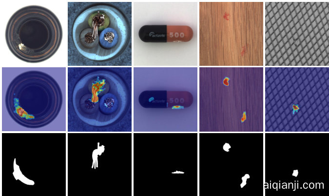
Figure 3. Visualization results on the MVTec AD [2] dataset under the zero-shot setting.
图 3: 零样本设置下在 MVTec AD [2] 数据集上的可视化结果。
As illustrated in the last three rows of Fig. 2, for simple categories, our method can effectively maintain the performance achieved in the zero-shot setting and achieve precise anomaly localization in the few-shot setting. For complex categories, our method, when combined with reference images, significantly reduces false detection rates. For example, in the case of macaroni in the 7th column, the extent of the anomalous region is narrowed down. Similarly, for PCB in the 10th column, the anomaly scores for normal components are greatly reduced.
如图 2 最后三行所示,对于简单类别,我们的方法能有效保持零样本 (zero-shot) 设定下的性能,并在少样本 (few-shot) 设定中实现精确的异常定位。针对复杂类别,当结合参考图像时,我们的方法能显著降低误检率。例如第 7 列的 macaroni 案例中,异常区域的范围被缩小;同样在第 10 列的 PCB 案例中,正常组件的异常评分大幅降低。
3.3. Quantitative results for VAND
3.3. VAND 定量结果
Due to the un availability of the ground-truth anomaly maps for the VAND test set, we present the top 5 results from the leader board for both tracks.
由于VAND测试集缺乏真实异常标注图,我们列出了两个赛道的排行榜前5名结果。
Zero-shot setting. As shown in the Tab. 1, our method achieved F1 scores of 0.3431 for anomaly segmentation and 0.7782 for anomaly classification in the zero-shot track, ranking first overall. Specifically, our method ranked first in the anomaly segmentation and fifth in the anomaly classification individually. Notebaly, our method significantly outperforms the second-ranked team in terms of segmentation, with a large margin of 0.0489.
零样本设置。如表 1 所示,我们的方法在零样本赛道中实现了异常分割 F1 分数 0.3431 和异常分类 F1 分数 0.7782,综合排名第一。具体而言,我们的方法在异常分割中排名第一,在异常分类中单独排名第五。值得注意的是,我们的方法在分割方面显著优于第二名团队,领先幅度高达 0.0489。
Few-shot setting. As to the few-shot track, although we only ranked fourth in the Tab. 2, it is notable that we ranked first in the anomaly classification with an F1 score of 0.8687. This score also considerably surpasses the secondranked team, exceeding them by 0.0207.
少样本设置。在少样本赛道上,尽管我们在表 2 中仅排名第四,但值得注意的是,我们在异常分类任务中以 0.8687 的 F1 分数位列第一。该分数远超第二名团队,领先优势达 0.0207。
3.4. Quantitative and qualitative results for MVTec
3.4. MVTec 的定量与定性结果
Tab. 3 presents the comparative results of our method and other approaches on the MVTec AD dataset. In the zero-shot setting, our method outperforms WinCLIP [8] by a large margin in terms of AUROC-segm $(2.5\uparrow)$ and F1- max-segm (11.6 ) metrics, but it achieves a lower PRO metric. We believe that this phenomenon may be related to the definition of the PRO metric. PRO essentially calculates the proportion of pixels successfully detected as anomalies within each connected component of anomalies. When the identified anomaly regions can completely cover the ground truth, or even exceed it, the PRO metric tends to be high. However, if the identified anomaly region is relatively small, even if its position is correct, the PRO metric may be lower. As shown in Fig. 3, our method tends to identify a precise anomaly region, which is often slightly smaller than the ground truth, despite being in the correct location. This could be attributed to training the linear layers on the VisA dataset, as compared to the MVTec AD dataset, anomalies in VisA tend to be smaller in size. As to anomaly classification, our method slightly lags behind WinCLIP.
表 3 展示了我们的方法与其他方法在 MVTec AD 数据集上的对比结果。在零样本设置下,我们的方法在 AUROC-segm $(2.5\uparrow)$ 和 F1-max-segm (11.6 ) 指标上大幅领先 WinCLIP [8],但在 PRO 指标上表现稍逊。我们认为这一现象可能与 PRO 指标的定义有关。PRO 本质上是计算每个异常连通分量中被成功检测为异常的像素比例。当识别出的异常区域能完全覆盖真实异常区域甚至超出时,PRO 指标往往较高。然而,如果识别出的异常区域相对较小,即使位置正确,PRO 指标也可能较低。如图 3 所示,我们的方法倾向于识别精确的异常区域,尽管位置正确,但通常略小于真实异常区域。这可能与在 VisA 数据集上训练线性层有关,因为相较于 MVTec AD 数据集,VisA 中的异常区域通常更小。在异常分类方面,我们的方法略逊于 WinCLIP。

Figure 4. Visualization results on the VisA [19] dataset under the zero-shot setting.
图 4: VisA [19] 数据集在零样本设置下的可视化结果。
In the few-shot setting, our method achieves slightly lower results compared to WinCLIP on most metrics, but significantly outperforms other comparison methods. Furthermore, in contrast to the zero-shot setting, our PRO metric surpasses that of WinCLIP, which can be attributed to the design of our multiple memory banks.
在少样本设置下,我们的方法在多数指标上略低于WinCLIP,但显著优于其他对比方法。此外,与零样本设置相比,我们的PRO指标超越了WinCLIP,这归功于多重记忆库的设计。
Additionally, the detailed results for each category in the MVTec AD dataset under the zero-shot, 1-shot, 2-shot, and 4-shot settings are recorded in Tab. 5, Tab. 6, Tab. 7 and Tab. 8, respectively.
此外,MVTec AD数据集中每个类别在零样本 (zero-shot)、1样本 (1-shot)、2样本 (2-shot) 和4样本 (4-shot) 设置下的详细结果分别记录在表5、表6、表7和表8中。
3.5. Quantitative and qualitative results for VisA
3.5. VisA 的定量与定性结果
Tab. 4 presents the comparative results of our method and other approaches on the VisA dataset. In the zero-shot setting, our method significantly outperforms WinCLIP [8] in metrics AUROC-segm (14.6 ), F1-max-segm $(17.5\uparrow)$ , and PRO-segm $(30\uparrow)$ . The visualization results are presented in Fig. 4. In this section, we trained on the MVTec AD dataset and tested on the VisA dataset. As the anomalies in MVTec AD tend to be larger overall, the detected anomaly regions on VisA also tend to be slightly larger than the ground truth, resulting in higher PRO scores. This is consistent with the discussion in Sec. 3.4. Although it slightly lags behind in anomaly classification, the difference is minimal, and in fact, our method even achieves a slightly higher AP metric compared to WinCLIP.
表 4 展示了我们的方法与其他方法在 VisA 数据集上的对比结果。在零样本设置下,我们的方法在指标 AUROC-segm (14.6↑)、F1-max-segm $(17.5\uparrow)$ 和 PRO-segm $(30\uparrow)$ 上显著优于 WinCLIP [8]。可视化结果如图 4 所示。本节中,我们在 MVTec AD 数据集上训练并在 VisA 数据集上测试。由于 MVTec AD 中的异常通常整体较大,因此在 VisA 上检测到的异常区域也往往比真实标注略大,导致 PRO 分数较高。这与第 3.4 节的讨论一致。虽然在异常分类方面稍显落后,但差异极小,事实上我们的方法甚至比 WinCLIP 获得了略高的 AP 指标。
Table 3. Quantitative comparisons on the MVTec AD [2] dataset. We report the mean and standard deviation over 5 random seeds for each measurement. Bold indicates the best performance, while underline denotes the second-best result.
表 3: MVTec AD [2] 数据集上的定量比较。我们报告了每个指标在 5 个随机种子上的均值和标准差。加粗表示最佳性能,下划线表示次优结果。
| 设置 | 方法 | AUROC-segm | F1-max-segm | AP-segm | PRO-segm | AUROC-cls | F1-max-cls | AP-cls |
|---|---|---|---|---|---|---|---|---|
| zero-shot | WinCLIP [8] | 85.1 | 31.7 | 64.6 | 91.8 | 92.9 | 96.5 | |
| Ours | 87.6 | 43.3 | 40.8 | 44.0 | 86.1 | 90.4 | 93.5 | |
| 1-shot | SPADE [4] | 92.0±0.3 | 44.5±1.0 | 85.7±0.7 | 82.9±2.6 | 91.1±1.0 | 91.7±1.2 | |
| PaDiM [5] | 91.3±0.7 | 43.7±1.5 | 78.2±1.8 | 78.9±3.1 | 89.2±1.1 | 89.3±1.7 | ||
| PatchCore [14] | 93.3±0.6 | 53.0±1.7 | 82.3±1.3 | 86.3±3.3 | 92.0±1.5 | 93.8±1.7 | ||
| WinCLIP [8] | 95.2±0.5 | 55.9±2.7 | 87.1±1.2 | 93.1±2.0 | 93.7±1.1 | 96.5±0.9 | ||
| Ours | 95.1±0.1 | 54.2±0.0 | 51.8±0.1 | 90.6±0.2 | 92.0±0.3 | 92.4±0.2 | 95.8±0.2 | |
| 2-shot | SPADE [4] | 91.2±0.4 | 42.4±1.0 | 83.9±0.7 | 81.0±2.0 | 90.3±0.8 | 90.6±0.8 | |
| PaDiM [5] | 89.3±0.9 | 40.2±2.1 | 73.3±2.0 | 76.6±3.1 | 88.2±1.1 | 88.1±1.7 | ||
| PatchCore [14] | 92.0±1.0 | 50.4±2.1 | 79.7±2.0 | 83.4±3.0 | 90.5±1.5 | 92.2±1.5 | ||
| WinCLIP [8] | 96.0±0.3 | 58.4±1.7 | 88.4±0.9 | 94.4±1.3 | 94.4±0.8 | 97.0±0.7 | ||
| Ours | 95.5±0.0 | 55.9±0.5 | 53.4±0.4 | 91.3±0.1 | 92.4±0.3 | 92.6±0.1 | 96.0±0.2 | |
| 4-shot | SPADE [4] | 92.7±0.3 | 46.2±1.3 | 87.0±0.5 | 84.8±2.5 | 91.5±0.9 | 92.5±1.2 | |
| PaDiM [5] | 92.6±0.7 | 46.1±1.8 | 81.3±1.9 | 80.4±2.5 | 90.2±1.2 | 90.5±1.6 | ||
| PatchCore [14] | 94.3±0.5 | 55.0±1.9 | 84.3±1.6 | 88.8±2.6 | 92.6±1.6 | 94.5±1.5 | ||
| WinCLIP [8] | 96.2±0.3 | 59.5±1.8 | 89.0±0.8 | 95.2±1.3 | 94.7±0.8 | 97.3±0.6 | ||
| Ours | 95.9±0.0 | 56.9±0.1 | 54.5±0.2 | 91.8±0.1 | 92.8±0.2 | 92.8±0.1 | 96.3±0.1 |
Table 4. Quantitative comparisons on the VisA [19] dataset. We report the mean and standard deviation over 5 random seeds for each measurement. Bold indicates the best performance, while underline denotes the second-best result.
表 4. VisA [19] 数据集上的定量比较。我们报告了每个测量指标在5个随机种子上的均值和标准差。加粗表示最佳性能,下划线表示次优结果。
| 设置 | 方法 | AUROC-segm | F1-max-segm | AP-segm | PRO-segm | AUROC-cls | F1-max-cls | AP-cls |
|---|---|---|---|---|---|---|---|---|
| 零样本 | WinCLIP [8] | 79.6 | 14.8 | 56.8 | 78.1 | 79.0 | 81.2 | |
| 零样本 | Ours | 94.2 | 32.3 | 25.7 | 86.8 | 78.0 | 78.7 | 81.4 |
| 1样本 | SPADE [4] | 95.6±0.4 | 35.5±2.2 | 84.1±1.6 | 79.5±4.0 | 80.7±1.9 | 82.0±3.3 | |
| 1样本 | PaDiM [5] | 89.9±0.8 | 17.4±1.7 | 64.3±2.4 | 62.8±5.4 | 75.3±1.2 | 68.3±4.0 | |
| 1样本 | PatchCore [14] | 95.4±0.6 | 38.0±1.9 | 80.5±2.5 | 79.9±2.9 | 81.7±1.6 | 82.8±2.3 | |
| 1样本 | WinCLIP [8] | 96.4±0.4 | 41.3±2.3 | 85.1±2.1 | 83.8±4.0 | 83.1±1.7 | 85.1±4.0 | |
| 1样本 | Ours | 96.0±0.0 | 38.5±0.3 | 30.9±0.3 | 90.0±0.1 | 91.2±0.8 | 86.9±0.6 | 93.3±0.8 |
| 2样本 | SPADE [4] | 96.2±0.4 | 40.5±3.7 | 85.7±1.1 | 80.7±5.0 | 81.7±2.5 | 82.3±4.3 | |
| 2样本 | PaDiM [5] | 92.0±0.7 | 21.1±2.4 | 70.1±2.6 | 67.4±5.1 | 75.7±1.8 | 71.6±3.8 | |
| 2样本 | PatchCore [14] | 96.1±0.5 | 41.0±3.9 | 82.6±2.3 | 81.6±4.0 | 82.5±1.8 | 84.8±3.2 | |
| 2样本 | WinCLIP [8] | 96.8±0.3 | 43.5±3.3 | 86.2±1.4 | 84.6±2.4 | 83.0±1.4 | 85.8±2.7 | |
| 2样本 | Ours | 96.2±0.0 | 39.3±0.2 | 31.6±0.3 | 90.1±0.1 | 92.2±0.3 | 87.7±0.3 | 94.2±0.3 |
| 4样本 | SPADE [4] | 96.6±0.3 | 43.6±3.6 | 87.3±0.8 | 81.7±3.4 | 82.1±2.1 | 83.4±2.7 | |
| 4样本 | PaDiM [5] | 93.2±0.5 | 24.6±1.8 | 72.6±1.9 | 72.8±2.9 | 78.0±1.2 | 75.6±2.2 | |
| 4样本 | PatchCore [14] | 96.8±0.3 | 43.9±3.1 | 84.9±1.4 | 85.3±2.1 | 84.3±1.3 | 87.5±2.1 | |
| 4样本 | WinCLIP [8] | 97.2±0.2 | 47.0±3.0 | 87.6±0.9 | 87.3±1.8 | 84.2±1.6 | 88.8±1.8 | |
| 4样本 | Ours | 96.2±0.0 | 40.0±0.1 | 32.2±0.1 | 90.2±0.1 | 92.6±0.4 | 88.4±0.5 | 94.5±0.3 |
In the few-shot setting, our method falls slightly behind WinCLIP in terms of anomaly segmentation, but achieves a higher PRO metric. It is worth noting that our method significantly outperforms WinCLIP and other methods in all metrics related to anomaly classification.
在少样本设置下,我们的方法在异常分割方面略逊于WinCLIP,但获得了更高的PRO指标。值得注意的是,我们的方法在所有与异常分类相关的指标上都显著优于WinCLIP及其他方法。
Additionally, the detailed results for each category in the VisA dataset under the zero-shot, 1-shot, 2-shot, and 4-shot settings are recorded in Tab. 9, Tab. 10, Tab. 11 and Tab. 12, respectively.
此外,VisA数据集中每个类别在零样本、1样本、2样本和4样本设置下的详细结果分别记录在表9、表10、表11和表12中。
4. Conclusion
4. 结论
In reality, due to the diverse range of industrial products, it is not feasible to collect a large number of training images or train specialized models for each category. Thus, designing joint models for zero/few-shot settings is a promising research direction. We made slight modifications to the CLIP model by adding extra linear layers, enabling it to perform zero-shot segmentation while still being capable of zeroshot classification. Moreover, we further improved the performance by incorporating memory banks along with a few reference images. Our approach achieved first place in the zero-shot track and fourth place in the few-shot track of the VAND Challenge.
现实中,由于工业产品种类繁多,为每个类别收集大量训练图像或训练专用模型并不可行。因此,设计适用于零样本/少样本场景的联合模型是一个有前景的研究方向。我们对CLIP模型进行了微调,通过添加额外线性层使其在保持零样本分类能力的同时实现零样本分割。此外,我们通过引入记忆库和少量参考图像进一步提升了性能。该方法在VAND挑战赛的零样本赛道获得第一名,少样本赛道获得第四名。
Acknowledgments. This work is support by the Youtu Lab, Tencent, and we appreciate the constructive advice and guidance provided by Yabiao Wang (Researcher in Youtu Lab, Tencent), Chengjie Wang (Researcher in Youtu Lab, Tencent), and Yong Liu (Prof. in APRIL Lab, Zhejiang University).
致谢。本工作由腾讯优图实验室支持,感谢腾讯优图实验室研究员王亚彪、王成杰以及浙江大学APRIL实验室教授刘勇提供的建设性意见与指导。
References
参考文献
Table 5. Quantitative results of the zero-shot setting on the MVTec AD [2] dataset.
表 5. MVTec AD [2] 数据集上零样本 (zero-shot) 设置的定量结果。
| Object | AUROC-segm | segm | F1-max-AP-segm | PRO-segm | AUROC-F1-max-cls | cls | AP-cls |
|---|---|---|---|---|---|---|---|
| carpet | 98.4 | 65.7 | 67.5 | 48.5 | 99.5 | 98.3 | 99.8 |
| bottle | 83.4 | 53.4 | 53.0 | 45.6 | 92.0 | 92.8 | 97.7 |
| hazelnut | 96.1 | 50.5 | 49.7 | 70.3 | 89.6 | 87.7 | 94.8 |
| leather | 99.1 | 50.0 | 52.3 | 72.4 | 99.7 | 98.9 | 99.9 |
| cable | 72.3 | 23.9 | 18.2 | 25.7 | 88.4 | 84.6 | 93.1 |
| capsule | 92.0 | 33.1 | 29.7 | 51.3 | 79.9 | 91.6 | 95.5 |
| grid | 95.8 | 40.7 | 36.6 | 31.6 | 86.3 | 89.1 | 94.9 |
| pill | 76.2 | 27.7 | 23.6 | 65.4 | 80.5 | 91.6 | 96.0 |
| transistor | 62.4 | 19.0 | 11.7 | 21.3 | 80.8 | 73.1 | 77.5 |
| metal_nut | 65.4 | 28.1 | 25.9 | 38.4 | 68.4 | 89.4 | 91.9 |
| screw | 97.8 | 41.7 | 33.7 | 67.1 | 84.9 | 89.3 | 93.6 |
| toothbrush | 95.8 | 48.1 | 43.2 | 54.5 | 53.8 | 83.3 | 71.5 |
| zipper | 91.1 | 40.5 | 38.7 | 10.7 | 89.6 | 90.8 | 97.1 |
| tile | 92.7 | 66.5 | 66.3 | 26.7 | 99.9 | 99.4 | 100.0 |
| wood | 95.8 | 60.3 | 61.8 | 31.1 | 99.0 | 96.8 | 99.7 |
| Mean | 87.6 | 43.3 | 40.8 | 44.0 | 86.1 | 90.4 | 93.5 |
Table 6. Quantitative results of the 1-shot setting on the MVTec AD [2] dataset. We report the mean and standard deviation over 5 random seeds for each measurement.
表 6: MVTec AD [2] 数据集上少样本 (1-shot) 设置的定量结果。我们报告了每个指标在5个随机种子上的均值和标准差。
| 对象 | AUROC-segm | F1-max-segm | AP-segm | PRO-segm | AUROC-cls | F1-max-cls | AP-cls |
|---|---|---|---|---|---|---|---|
| carpet | 98.7±0.0 | 71.6±0.2 | 71.6±0.1 | 96.5±0.2 | 99.9±0.0 | 99.0±0.2 | 100.0±0.0 |
| bottle | 96.4±0.1 | 71.6±0.8 | 73.7±0.7 | 92.7±0.1 | 92.8±0.3 | 92.3±1.1 | 97.8±0.1 |
| hazelnut | 97.6±0.1 | 59.2±1.2 | 59.3±1.2 | 92.1±0.3 | 98.5±0.1 | 96.8±0.3 | 99.3±0.0 |
| leather | 99.5±0.0 | 51.6±0.3 | 55.9±0.1 | 99.0±0.1 | 99.9±0.1 | 99.6±0.2 | 100.0±0.0 |
| cable | 90.8±0.5 | 36.3±1.4 | 31.6±0.8 | 81.5±1.3 | 74.7±1.2 | 78.2±0.4 | 84.8±0.9 |
| capsule | 97.1±0.3 | 37.0±4.2 | 36.3±3.8 | 95.6±0.7 | 92.0±2.2 | 92.8±0.4 | 98.3±0.6 |
| grid | 96.9±0.3 | 47.7±1.2 | 41.8±0.9 | 90.2±0.7 | 99.0±0.3 | 98.1±0.8 | 99.6±0.1 |
| pill | 94.8±0.5 | 54.4±1.1 | 46.4±1.3 | 96.6±0.2 | 84.6±0.7 | 92.4±0.2 | 97.0±0.2 |
| transistor | 80.4±1.4 | 35.5±2.6 | 25.5±1.9 | 64.8±1.4 | 83.4±1.2 | 75.0±1.5 | 76.1±2.6 |
| metal_nut | 89.6±0.9 | 54.1±2.0 | 53.1±2.0 | 88.2±0.8 | 88.5±1.2 | 90.6±0.6 | 97.4±0.3 |
| screw | 98.2±0.0 | 42.1±0.7 | 34.4±0.5 | 92.6±0.2 | 79.8±0.6 | 88.4±0.2 | 91.1±0.4 |
| toothbrush | 98.4±0.3 | 55.3±1.2 | 55.1±1.8 | 93.4±1.1 | 94.3±2.1 | 93.0±1.5 | 97.8±0.8 |
| zipper | 96.1±0.2 | 56.3±0.9 | 54.6±1.0 | 87.2±0.7 | 94.3±0.3 | 94.6±0.7 | 98.3±0.1 |
| tile | 95.4±0.2 | 72.0±0.5 | 69.4±0.5 | 92.3±0.3 | 98.9±0.1 | 97.4±0.3 | 99.6±0.0 |
| wood | 96.1±0.1 | 67.9±0.3 | 69.0±0.5 | 95.9±0.1 | 98.5±0.1 | 97.5±0.0 | 99.5±0.0 |
| Mean | 95.1±0.1 | 54.2±0.0 | 51.8±0.1 | 90.6±0.2 | 92.0±0.3 | 92.4±0.2 | 95.8±0.2 |
Table 7. Quantitative results of the 2-shot setting on the MVTec AD [2] dataset. We report the mean and standard deviation over 5 random seeds for each measurement.
表 7: MVTec AD [2] 数据集上 2-shot 设置的定量结果。我们报告了每个指标在 5 个随机种子上的均值和标准差。
| Object | AUROC-segm | F1-max-segm | AP-segm | PRO-segm | AUROC-cls | F1-max-cls | AP-cls |
|---|---|---|---|---|---|---|---|
| carpet | 98.7±0.0 | 71.7±0.1 | 71.7±0.1 | 96.7±0.1 | 99.9±0.0 | 99.0±0.2 | 100.0±0.0 |
| bottle | 96.9±0.1 | 73.3±0.7 | 75.6±0.6 | 93.6±0.2 | 94.0±0.4 | 93.2±0.4 | 98.2±0.1 |
| hazelnut | 97.7±0.1 | 60.6±0.3 | 60.8±0.7 | 92.5±0.2 | 98.7±0.1 | 97.1±0.4 | 99.4±0.1 |
| leather | 99.5±0.0 | 51.5±0.2 | 56.0±0.1 | 99.0±0.1 | 100.0±0.0 | 99.8±0.2 | 100.0±0.0 |
| cable | 91.2±0.8 | 38.9±0.9 | 33.1±0.7 | 82.9±0.8 | 74.9±1.0 | 78.2±0.9 | 85.1±0.8 |
| capsule | 97.1±0.3 | 39.2±4.9 | 38.2±4.5 | 96.0±0.9 | 92.1±2.1 | 92.9±0.5 | 98.4±0.5 |
| grid | 96.9±0.2 | 48.7±0.6 | 42.2±0.4 | 90.9±0.8 | 99.0±0.1 | 97.7±0.4 | 99.6±0.0 |
| pill | 95.0±0.3 | 55.2±0.8 | 47.0±0.9 | 96.7±0.2 | 84.1±0.2 | 92.4±0.2 | 96.9±0.1 |
| transistor | 82.5±0.5 | 38.5±1.5 | 27.9±1.0 | 66.5±0.6 | 83.8±0.7 | 74.8±1.8 | 77.5±1.7 |
| metal_nut | 92.1±0.5 | 62.5±2.3 | 60.7±2.0 | 90.5±0.4 | 90.5±0.3 | 91.9±0.6 | 97.8±0.0 |
| screw | 98.3±0.1 | 43.2±0.4 | 36.2±1.1 | 93.1±0.6 | 82.0±2.2 | 88.8±0.3 | 92.4±1.4 |
| toothbrush | 98.5±0.2 | 55.6±0.7 | 55.9±1.3 | 93.8±0.5 | 94.8±1.3 | 93.3±0.5 | 98.0±0.5 |
| zipper | 96.4±0.1 | 59.2±0.7 | 57.2±0.6 | 88.7±0.5 | 94.7±0.5 | 94.7±0.5 | 98.4±0.2 |
| tile | 95.8±0.1 | 72.3±0.2 | 69.9±0.3 | 92.3±0.3 | 99.0±0.1 | 97.7±0.0 | 99.6±0.0 |
| wood | 96.1±0.1 | 67.7±0.3 | 68.8±0.3 | 96.0±0.1 | 98.7±0.3 | 97.5±0.0 | 99.6±0.1 |
| Mean | 95.5±0.0 | 55.9±0.5 | 53.4±0.4 | 91.3±0.1 | 92.4±0.3 | 92.6±0.1 | 96.0±0.2 |
Table 8. Quantitative results of the 4-shot setting on the MVTec AD [2] dataset. We report the mean and standard deviation over 5 random seeds for each measurement.
表 8. MVTec AD [2] 数据集上 4-shot 设置的定量结果。我们报告了每个测量指标在 5 个随机种子上的均值和标准差。
| Object | AUROC-segm | F1-max-segm | AP-segm | PRO-segm | AUROC-cls | F1-max-cls | AP-cls |
|---|---|---|---|---|---|---|---|
| carpet | 98.7±0.0 | 71.8±0.1 | 71.8±0.1 | 96.6±0.2 | 99.9±0.0 | 99.0±0.2 | 100.0±0.0 |
| bottle | 97.2±0.1 | 74.1±0.6 | 76.5±0.5 | 94.3±0.3 | 94.2±0.2 | 93.3±0.4 | 98.3±0.0 |
| hazelnut | 97.7±0.1 | 60.5±0.4 | 60.7±0.5 | 92.6±0.2 | 98.8±0.1 | 97.1±0.4 | 99.4±0.1 |
| leather | 99.5±0.0 | 51.5±0.1 | 55.9±0.1 | 98.9±0.1 | 100.0±0.0 | 99.9±0.2 | 100.0±0.0 |
| cable | 91.8±0.7 | 41.2±0.7 | 34.5±0.5 | 84.0±0.8 | 76.7±0.8 | 79.0±0.5 | 86.5±0.5 |
| capsule | 97.5±0.2 | 42.2±0.6 | 41.0±0.5 | 96.6±0.3 | 93.5±0.8 | 93.3±0.6 | 98.7±0.2 |
| grid | 97.6±0.3 | 49.0±0.9 | 43.4±1.0 | 92.0±0.8 | 99.2±0.2 | 98.1±0.3 | 99.7±0.1 |
| pill | 95.5±0.2 | 56.3±0.2 | 48.2±0.5 | 96.7±0.1 | 84.1±0.9 | 92.3±0.1 | 96.9±0.2 |
| transistor | 83.7±1.0 | 40.0±2.2 | 29.2±1.8 | 67.7±1.4 | 84.1±1.0 | 74.4±0.5 | 78.1±1.5 |
| metal_nut | 93.1±0.7 | 66.7±3.0 | 64.2±2.4 | 91.7±0.7 | 91.0±0.4 | 92.2±0.6 | 97.9±0.1 |
| screw | 98.5±0.2 | 43.7±1.2 | 37.7±2.2 | 93.7±0.3 | 83.7±2.3 | 89.5±0.7 | 93.2±1.7 |
| toothbrush | 98.8±0.1 | 55.7±0.8 | 56.8±1.0 | 94.8±0.9 | 93.2±0.7 | 92.6±0.6 | 97.3±0.3 |
| zipper | 96.6±0.1 | 60.2±1.0 | 58.2±0.9 | 89.2±0.5 | 95.4±0.4 | 95.7±0.8 | 98.6±0.1 |
| tile | 96.0±0.1 | 72.5±0.2 | 70.2±0.2 | 92.4±0.2 | 99.1±0.0 | 97.8±0.2 | 99.6±0.0 |
| wood | 96.2±0.0 | 67.7±0.2 | 69.0±0.2 | 96.1±0.2 | 98.7±0.2 | 97.5±0.0 | 99.6±0.1 |
| Mean | 95.9±0.0 | 56.9±0.1 | 54.5±0.2 | 91.8±0.1 | 92.8±0.2 | 92.8±0.1 | 96.3±0.1 |
Table 9. Quantitative results of the zero-shot setting on the VisA [19] dataset.
表 9. VisA [19] 数据集上零样本 (Zero-shot) 设置的定量结果
| Object | AUROC-segm | segm | F1-max-AP-segm | PRO-segm | AUROC-F1-max-cls | cls | AP-cls |
|---|---|---|---|---|---|---|---|
| candle | 97.8 | 39.4 | 29.9 | 92.5 | 83.8 | 77.8 | 86.9 |
| capsules | 97.5 | 48.5 | 40.0 | 86.7 | 61.2 | 77.6 | 74.3 |
| cashew | 86.0 | 22.9 | 15.1 | 91.7 | 87.3 | 84.8 | 94.1 |
| chewinggum | 99.5 | 78.5 | 83.6 | 87.3 | 96.4 | 93.7 | 98.4 |
| fryum | 92.0 | 29.7 | 22.1 | 89.7 | 94.3 | 91.7 | 97.2 |
| macaronil | 98.8 | 35.5 | 24.8 | 93.2 | 71.6 | 71.1 | 70.9 |
| macaroni2 | 97.8 | 13.7 | 6.8 | 82.3 | 64.6 | 69.1 | 63.2 |
| pcb1 | 92.7 | 12.5 | 8.4 | 87.5 | 53.4 | 66.9 | 57.2 |
| pcb2 | 89.7 | 23.4 | 15.4 | 75.6 | 71.8 | 70.1 | 73.8 |
| pcb3 | 88.4 | 21.7 | 14.1 | 77.8 | 66.8 | 66.7 | 70.7 |
| pcb4 | 94.6 | 31.3 | 24.9 | 86.8 | 95.0 | 87.3 | 95.1 |
| pipe_fryum | 96.0 | 30.4 | 23.6 | 90.9 | 89.9 | 87.7 | 94.8 |
| Mean | 94.2 | 32.3 | 25.7 | 86.8 | 78.0 | 78.7 | 81.4 |
Table 10. Quantitative results of the 1-shot setting on the VisA [19] dataset. We report the mean and standard deviation over 5 random seeds for each measurement.
表 10: VisA [19] 数据集上少样本 (1-shot) 设置的定量结果。我们报告了每个测量指标在5个随机种子上的均值和标准差。
| 物体 | AUROC-segm | F1-max-segm | AP-segm | PRO-segm | AUROC-cls | F1-max-cls | AP-cls |
|---|---|---|---|---|---|---|---|
| candle | 98.7±0.1 | 42.4±0.3 | 29.7±1.4 | 96.4±0.2 | 90.9±0.5 | 84.3±0.9 | 91.6±0.7 |
| capsules | 98.0±0.0 | 51.8±0.2 | 45.3±0.4 | 88.4±0.1 | 92.7±1.0 | 90.2±1.0 | 95.8±0.7 |
| cashew | 90.8±0.1 | 30.9±0.5 | 23.1±0.5 | 94.2±0.2 | 93.4±1.0 | 90.7±0.9 | 97.1±0.5 |
| chewinggum | 99.7±0.0 | 78.8±0.3 | 82.2±0.5 | 92.1±0.2 | 97.3±0.1 | 97.1±0.4 | 99.0±0.0 |
| fryum | 93.6±0.1 | 33.5±0.2 | 25.9±0.2 | 91.5±0.3 | 93.4±0.7 | 91.9±0.8 | 97.3±0.3 |
| macaronil | 99.3±0.0 | 37.2±0.2 | 26.5±0.5 | 95.3±0.1 | 89.7±0.6 | 82.5±0.8 | 92.0±0.4 |
| macaroni2 | 98.4±0.1 | 22.5±1.9 | 11.5±1.2 | 85.6±0.7 | 79.2±3.8 | 72.9±2.2 | 83.4±3.2 |
| pcb1 | 95.3±0.1 | 20.6±1.6 | 15.8±0.8 | 90.4±0.6 | 89.0±7.3 | 81.6±6.0 | 90.2±5.5 |
| pcb2 | 92.5±0.1 | 31.5±0.9 | 20.5±1.4 | 79.2±0.3 | 85.4±6.5 | 79.8±3.5 | 87.1±7.8 |
| pcb3 | 93.2±0.0 | 38.5±1.1 | 28.1±1.7 | 81.3±0.2 | 87.8±1.2 | 82.0±1.3 | 89.4±1.2 |
| pcb4 | 95.8±0.1 | 37.6±0.9 | 32.6±1.3 | 89.3±0.3 | 97.5±0.3 | 93.7±0.7 | 97.0±0.5 |
| pipe_fryum | 97.3±0.0 | 36.6±0.3 | 29.6±0.5 | 96.1±0.1 | 98.3±0.4 | 96.3±0.6 | 99.2±0.2 |
| Mean | 96.0±0.0 | 38.5±0.3 | 30.9±0.3 | 90.0±0.1 | 91.2±0.8 | 86.9±0.6 | 93.3±0.8 |
Table 11. Quantitative results of the 2-shot setting on the VisA [19] dataset. We report the mean and standard deviation over 5 random seeds for each measurement.
表 11: VisA [19] 数据集上 2-shot 设置的定量结果。我们报告了每个指标在 5 个随机种子上的均值和标准差。
| 物体 | AUROC-segm | F1-max-segm | AP-segm | PRO-segm | AUROC-cls | Fl-max-cls | AP-cls |
|---|---|---|---|---|---|---|---|
| candle | 98.6±0.1 | 42.4±0.3 | 29.5±1.6 | 96.5±0.2 | 91.3±0.5 | 84.3±0.4 | 91.9±0.6 |
| capsules | 98.0±0.0 | 52.2±0.2 | 45.7±0.3 | 89.1±0.3 | 93.4±0.3 | 90.4±0.7 | 96.3±0.2 |
| cashew | 90.8±0.1 | 31.4±0.4 | 23.4±0.5 | 94.1±0.2 | 93.4±0.6 | 91.6±0.5 | 97.2±0.3 |
| chewinggum | 99.7±0.0 | 78.8±0.3 | 82.4±0.3 | 92.1±0.3 | 97.1±0.1 | 96.9±0.4 | 98.9±0.0 |
| fryum | 93.6±0.0 | 34.0±0.1 | 26.3±0.1 | 91.6±0.1 | 93.1±0.4 | 91.5±0.7 | 97.2±0.1 |
| macaronil | 99.3±0.0 | 37.0±0.4 | 26.3±0.7 | 95.2±0.1 | 90.0±0.4 | 82.5±0.4 | 92.1±0.2 |
| macaroni2 | 98.4±0.0 | 24.2±0.8 | 12.3±0.6 | 85.4±0.2 | 81.0±1.0 | 74.1±1.1 | 85.1±0.9 |
| pcb1 | 95.8±0.2 | 24.2±3.2 | 18.9±2.4 | 90.6±0.2 | 90.9±1.3 | 83.8±0.8 | 91.6±0.9 |
| pcb2 | 92.8±0.1 | 32.6±0.4 | 21.6±0.3 | 79.7±0.3 | 89.2±1.5 | 83.3±1.7 | 91.3±1.2 |
| pcb3 | 93.5±0.0 | 40.5±0.8 | 30.6±1.0 | 81.5±0.5 | 90.9±0.8 | 84.5±1.2 | 92.2±0.7 |
| pcb4 | 95.9±0.1 | 38.3±0.5 | 33.0±0.8 | 89.5±0.3 | 97.9±0.5 | 93.1±1.1 | 97.8±0.6 |
| pipe_fryum | 97.3±0.0 | 36.8±0.2 | 29.8±0.3 | 96.1±0.3 | 98.4±0.2 | 96.2±0.6 | 99.3±0.1 |
| Mean | 96.2±0.0 | 39.3±0.2 | 31.6±0.3 | 90.1±0.1 | 92.2±0.3 | 87.7±0.3 | 94.2±0.3 |
Table 12. Quantitative results of the 4-shot setting on the VisA [19] dataset. We report the mean and standard deviation over 5 random seeds for each measurement.
表 12. VisA [19] 数据集上 4-shot 设置的定量结果。我们报告了每个测量指标在 5 个随机种子上的均值和标准差。
| 对象 | AUROC-segm | F1-max-segm | AP-segm | PRO-segm | AUROC-cls | F1-max-cls | AP-cls |
|---|---|---|---|---|---|---|---|
| candle | 98.7±0.0 | 42.4±0.2 | 29.6±1.0 | 96.3±0.1 | 91.4±0.5 | 85.1±0.5 | 92.0±0.6 |
| capsules | 98.1±0.0 | 52.4±0.3 | 46.0±0.5 | 89.0±0.4 | 93.7±0.1 | 90.6±0.4 | 96.5±0.1 |
| cashew | 90.8±0.1 | 31.6±0.3 | 23.7±0.3 | 94.1±0.2 | 94.3±0.3 | 92.2±0.5 | 97.6±0.2 |
| chewinggum | 99.7±0.0 | 78.8±0.3 | 82.0±0.2 | 92.2±0.3 | 97.2±0.2 | 97.2±0.2 | 99.0±0.0 |
| fryum | 93.7±0.0 | 34.2±0.0 | 26.4±0.0 | 91.5±0.1 | 93.5±0.5 | 92.3±1.2 | 97.4±0.2 |
| macaronil | 99.3±0.0 | 37.3±0.4 | 27.2±0.5 | 95.2±0.1 | 90.1±0.4 | 82.7±0.7 | 92.4±0.3 |
| macaroni2 | 98.4±0.0 | 24.6±0.4 | 12.5±0.4 | 85.8±0.2 | 82.5±0.5 | 76.2±0.8 | 86.3±0.3 |
| pcb1 | 96.0±0.0 | 27.7±1.1 | 21.7±0.7 | 90.6±0.1 | 91.2±1.5 | 85.2±1.8 | 91.8±1.0 |
| pcb2 | 93.0±0.1 | 32.4±0.6 | 21.8±0.4 | 80.2±0.3 | 89.2±0.7 | 82.6±1.7 | 91.3±0.7 |
| pcb3 | 93.7±0.1 | 41.9±0.4 | 31.4±0.6 | 81.5±0.3 | 91.6±0.4 | 85.7±0.7 | 92.7±0.3 |
| pcb4 | 96.0±0.0 | 39.2±0.3 | 34.1±0.3 | 89.7±0.1 | 98.2±0.3 | 94.1±0.3 | 98.0±0.3 |
| pipe_fryum | 97.4±0.0 | 36.8±0.3 | 30.0±0.3 | 95.9±0.2 | 98.5±0.4 | 96.8±0.7 | 99.4±0.2 |
| Mean | 96.2±0.0 | 40.0±0.1 | 32.2±0.1 | 90.2±0.1 | 92.6±0.4 | 88.4±0.5 | 94.5±0.3 |