Group Normalization
组归一化 (Group Normalization)
Yuxin Wu Kaiming He
吴育昕 何恺明
Facebook AI Research (FAIR) {yuxinwu,kaiminghe}@fb.com
Facebook AI Research (FAIR) {yuxinwu,kaiminghe}@fb.com
Abstract
摘要
Batch Normalization (BN) is a milestone technique in the development of deep learning, enabling various networks to train. However, normalizing along the batch dimension introduces problems — BN’s error increases rapidly when the batch size becomes smaller, caused by inaccurate batch statistics estimation. This limits BN’s usage for training larger models and transferring features to computer vision tasks including detection, segmentation, and video, which require small batches constrained by memory consumption. In this paper, we present Group Normalization (GN) as a simple alternative to BN. GN divides the channels into groups and computes within each group the mean and variance for normalization. GN’s computation is independent of batch sizes, and its accuracy is stable in a wide range of batch sizes. On ResNet-50 trained in ImageNet, GN has $10.6%$ lower error than its BN counterpart when using a batch size of 2; when using typical batch sizes, GN is comparably good with BN and outperforms other normalization variants. Moreover, GN can be naturally transferred from pre-training to fine-tuning. GN can outperform its BNbased counterparts for object detection and segmentation in COCO,1 and for video classification in Kinetics, showing that GN can effectively replace the powerful BN in a variety of tasks. GN can be easily implemented by a few lines of code in modern libraries.
批归一化 (Batch Normalization, BN) 是深度学习发展中的里程碑技术,它使得各种网络能够进行训练。然而,沿批次维度进行归一化会带来问题——当批次规模变小时,由于批次统计量估计不准确,BN 的误差会迅速增大。这限制了 BN 在训练更大模型以及将特征迁移到计算机视觉任务(包括检测、分割和视频处理)中的应用,这些任务受内存消耗限制而需要使用小批次。本文提出组归一化 (Group Normalization, GN) 作为 BN 的简单替代方案。GN 将通道划分为若干组,并在每组内计算均值和方差以进行归一化。GN 的计算与批次规模无关,其精度在广泛的批次规模范围内保持稳定。在 ImageNet 上训练的 ResNet-50 中,当批次规模为 2 时,GN 的误差比 BN 低 10.6%;在使用典型批次规模时,GN 与 BN 表现相当,并优于其他归一化变体。此外,GN 可以自然地从预训练迁移到微调。在 COCO 的目标检测和分割任务中,以及在 Kinetics 的视频分类任务中,GN 的表现优于基于 BN 的方案,这表明 GN 可以在多种任务中有效替代强大的 BN。GN 只需在现代库中用几行代码即可轻松实现。
1. Introduction
1. 引言
Batch Normalization (Batch Norm or BN) [26] has been established as a very effective component in deep learning, largely helping push the frontier in computer vision [59, 20] and beyond [54]. BN normalizes the features by the mean and variance computed within a (mini-)batch. This has been shown by many practices to ease optimization and enable very deep networks to converge. The stochastic uncertainty of the batch statistics also acts as a regularize r that can benefit generalization. BN has been a foundation of many stateof-the-art computer vision algorithms.
批归一化 (Batch Normalization 或 BN) [26] 已成为深度学习中非常有效的组件,极大地推动了计算机视觉 [59, 20] 及其他领域 [54] 的发展。BN 通过计算(小)批次内的均值和方差对特征进行归一化。许多实践表明,这种方法可以简化优化过程并使极深度网络收敛。批次统计的随机不确定性还起到了正则化作用,有助于提升泛化性能。BN 已成为众多最先进计算机视觉算法的基础。
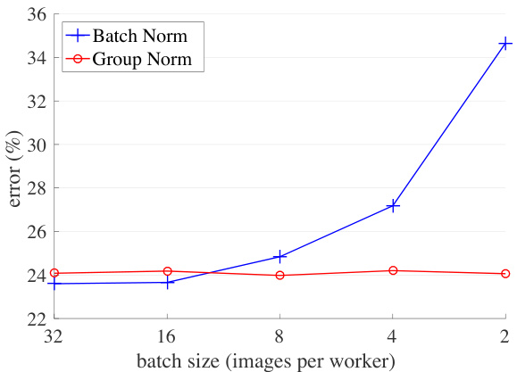
Figure 1. ImageNet classification error vs. batch sizes. This is a ResNet-50 model trained in the ImageNet training set using 8 workers (GPUs), evaluated in the validation set.
图 1: ImageNet分类错误率与批次大小的关系。该图展示了一个在ImageNet训练集上使用8个工作节点(GPU)训练的ResNet-50模型,并在验证集上进行评估的结果。
Despite its great success, BN exhibits drawbacks that are also caused by its distinct behavior of normalizing along the batch dimension. In particular, it is required for BN to work with a sufficiently large batch size (e.g., 32 per worker2 [26, 59, 20]). A small batch leads to inaccurate estimation of the batch statistics, and reducing BN’s batch size increases the model error dramatically (Figure 1). As a result, many recent models [59, 20, 57, 24, 63] are trained with non-trivial batch sizes that are memory-consuming. The heavy reliance on BN’s effectiveness to train models in turn prohibits people from exploring higher-capacity models that would be limited by memory.
尽管取得了巨大成功,批量归一化(BN)仍存在因其沿批次维度归一化的独特行为而导致的缺陷。具体而言,BN需要足够大的批次量才能有效工作(例如每个worker需32个样本 [26, 59, 20])。小批次量会导致批次统计量估计不准确,降低BN的批次量会显著增加模型误差(图1)。因此,许多最新模型[59, 20, 57, 24, 63]都采用内存消耗可观的大批次量进行训练。这种对BN效能的严重依赖反过来阻碍了研究者探索受内存限制的更高容量模型。
The restriction on batch sizes is more demanding in computer vision tasks including detection [12, 47, 18], segmentation [38, 18], video recognition [60, 6], and other highlevel systems built on them. For example, the Fast/er and Mask R-CNN frameworks [12, 47, 18] use a batch size of 1 or 2 images because of higher resolution, where BN is “frozen” by transforming to a linear layer [20]; in video classification with 3D convolutions [60, 6], the presence of spatial-temporal features introduces a trade-off between the temporal length and batch size. The usage of BN often requires these systems to compromise between the model design and batch sizes.
在计算机视觉任务中,包括检测 [12, 47, 18]、分割 [38, 18]、视频识别 [60, 6] 以及基于这些任务构建的其他高级系统,对批处理大小的限制更为严格。例如,Fast/er 和 Mask R-CNN 框架 [12, 47, 18] 由于分辨率较高,通常使用 1 或 2 张图像的批处理大小,此时 BN (Batch Normalization) 会通过转换为线性层 [20] 而被“冻结”;在采用 3D 卷积的视频分类任务中 [60, 6],时空特征的存在使得时间长度与批处理大小之间需要权衡。BN 的使用往往迫使这些系统在模型设计和批处理大小之间做出妥协。
This paper presents Group Normalization (GN) as a simple alternative to BN. We notice that many classical features like SIFT [39] and HOG [9] are group-wise features and involve group-wise normalization. For example, a HOG vector is the outcome of several spatial cells where each cell is represented by a normalized orientation histogram. Analogously, we propose GN as a layer that divides channels into groups and normalizes the features within each group (Figure 2). GN does not exploit the batch dimension, and its computation is independent of batch sizes.
本文提出了组归一化 (Group Normalization, GN) 作为批量归一化 (BN) 的简单替代方案。我们注意到 SIFT [39] 和 HOG [9] 等经典特征都是分组特征,并涉及分组归一化。例如,HOG 向量是多个空间单元的结果,其中每个单元由归一化的方向直方图表示。类似地,我们提出 GN 作为一种将通道划分为组并对每组特征进行归一化的层 (图 2)。GN 不利用批次维度,其计算与批次大小无关。
GN behaves very stably over a wide range of batch sizes (Figure 1). With a batch size of 2 samples, GN has $10.6%$ lower error than its BN counterpart for ResNet-50 [20] in ImageNet [50]. With a regular batch size, GN is comparably good as BN (with a gap of ${\sim}0.5%,$ ) and outperforms other normalization variants [3, 61, 51]. Moreover, although the batch size may change, GN can naturally transfer from pretraining to fine-tuning. GN shows improved results vs. its BN counterpart on Mask R-CNN for COCO object detection and segmentation [37], and on 3D convolutional net- works for Kinetics video classification [30]. The effectiveness of GN in ImageNet, COCO, and Kinetics demonstrates that GN is a competitive alternative to BN that has been dominant in these tasks.
GN在广泛的批量大小范围内表现非常稳定(图1)。当批量大小为2个样本时,在ImageNet[50]的ResNet-50[20]上,GN比对应的BN方法误差降低了10.6%。在常规批量大小下,GN与BN性能相当(差距约0.5%),并优于其他归一化变体[3,61,51]。此外,尽管批量大小可能变化,GN能够自然地实现从预训练到微调的迁移。在COCO目标检测与分割的Mask R-CNN[37]以及Kinetics视频分类的3D卷积网络[30]上,GN相比对应的BN方法都显示出更好的结果。GN在ImageNet、COCO和Kinetics上的有效性表明,GN是这些任务中占主导地位的BN的有力替代方案。
There have been existing methods, such as Layer Normalization (LN) [3] and Instance Normalization (IN) [61] (Figure 2), that also avoid normalizing along the batch dimension. These methods are effective for training sequential models (RNN/LSTM [49, 22]) or generative models (GANs [15, 27]). But as we will show by experiments, both LN and IN have limited success in visual recognition, for which GN presents better results. Conversely, GN could be used in place of LN and IN and thus is applicable for sequential or generative models. This is beyond the focus of this paper, but it is suggestive for future research.
现有方法如层归一化 (Layer Normalization, LN) [3] 和实例归一化 (Instance Normalization, IN) [61] (图 2) 也避免了沿批次维度进行归一化。这些方法对训练序列模型 (RNN/LSTM [49, 22]) 或生成模型 (GAN [15, 27]) 有效。但如实验所示,LN 和 IN 在视觉识别任务中效果有限,而组归一化 (GN) 表现更优。反之,GN 可替代 LN 和 IN,因此也适用于序列或生成模型。这虽非本文重点,但为未来研究提供了方向。
2. Related Work
2. 相关工作
Normalization. It is well-known that normalizing the input data makes training faster [33]. To normalize hidden features, initialization methods [33, 14, 19] have been derived based on strong assumptions of feature distributions, which can become invalid when training evolves.
归一化 (Normalization)。众所周知,对输入数据进行归一化可以加快训练速度 [33]。为了归一化隐藏特征,初始化方法 [33, 14, 19] 是基于特征分布的强假设推导而来的,这些假设在训练过程中可能会失效。
Normalization layers in deep networks had been widely used before the development of BN. Local Response Normalization (LRN) [40, 28, 32] was a component in AlexNet [32] and following models [64, 53, 58]. Unlike recent methods [26, 3, 61], LRN computes the statistics in a small neighborhood for each pixel.
深度网络中的归一化层在BN(批归一化)出现之前已被广泛使用。局部响应归一化(Local Response Normalization,LRN)[40, 28, 32]是AlexNet[32]及后续模型[64, 53, 58]的组成部分。与近期方法[26, 3, 61]不同,LRN针对每个像素在小邻域内计算统计量。
Batch Normalization [26] performs more global normalization along the batch dimension (and as importantly, it suggests to do this for all layers). But the concept of “batch” is not always present, or it may change from time to time. For example, batch-wise normalization is not legitimate at inference time, so the mean and variance are pre-computed from the training set [26], often by running average; consequently, there is no normalization performed when testing. The pre-computed statistics may also change when the target data distribution changes [45]. These issues lead to inconsistency at training, transferring, and testing time. In addition, as aforementioned, reducing the batch size can have dramatic impact on the estimated batch statistics.
批归一化 (Batch Normalization) [26] 沿批次维度执行更全局的归一化(同样重要的是,它建议对所有层都这样做)。但"批次"的概念并不总是存在,或者可能不时变化。例如,在推理时进行批次归一化是不合理的,因此均值和方差是从训练集[26]预先计算的,通常通过运行平均值;因此,在测试时没有执行归一化。当目标数据分布发生变化时,预先计算的统计量也可能发生变化[45]。这些问题导致训练、迁移和测试时的不一致性。此外,如前所述,减小批次大小会对估计的批次统计量产生巨大影响。
Several normalization methods [3, 61, 51, 2, 46] have been proposed to avoid exploiting the batch dimension. Layer Normalization (LN) [3] operates along the channel dimension, and Instance Normalization (IN) [61] per- forms BN-like computation but only for each sample (Figure 2). Instead of operating on features, Weight Normalization (WN) [51] proposes to normalize the filter weights. These methods do not suffer from the issues caused by the batch dimension, but they have not been able to approach BN’s accuracy in many visual recognition tasks. We provide comparisons with these methods in context of the remaining sections.
为避免利用批次维度,已提出了多种归一化方法 [3, 61, 51, 2, 46]。层归一化 (LN) [3] 沿通道维度操作,而实例归一化 (IN) [61] 执行类似 BN 的计算但仅针对每个样本 (图 2)。权重归一化 (WN) [51] 则提出对滤波器权重进行归一化,而非直接操作特征。这些方法不会受批次维度引发的问题影响,但在许多视觉识别任务中仍无法达到 BN 的准确度。我们将在后续章节中与这些方法进行对比。
Addressing small batches. Ioffe [25] proposes Batch Re normalization (BR) that alleviates BN’s issue involving small batches. BR introduces two extra parameters that constrain the estimated mean and variance of BN within a certain range, reducing their drift when the batch size is small. BR has better accuracy than BN in the small-batch regime. But BR is also batch-dependent, and when the batch size decreases its accuracy still degrades [25].
解决小批量问题。Ioffe [25] 提出了批量重归一化 (BR) 方法,缓解了 BN 在小批量场景下的问题。BR 引入了两个额外参数,将 BN 估计的均值和方差约束在一定范围内,从而减少小批量时这些统计量的漂移。在小批量情况下,BR 比 BN 具有更高的准确率。但 BR 同样依赖于批量大小,当批量减小时其准确率仍会下降 [25]。
There are also attempts to avoid using small batches. The object detector in [43] performs synchronized BN whose mean and variance are computed across multiple GPUs. However, this method does not solve the problem of small batches; instead, it migrates the algorithm problem to engineering and hardware demands, using a number of GPUs proportional to BN’s requirements. Moreover, the synchronized BN computation prevents using asynchronous solvers (ASGD [10]), a practical solution to large-scale training widely used in industry. These issues can limit the scope of using synchronized BN.
也有尝试避免使用小批量的方法。[43]中的目标检测器采用同步BN (Batch Normalization),其均值和方差通过多块GPU计算得出。然而这种方法并未解决小批量问题,而是将算法问题转化为工程和硬件需求,需要使用与BN要求数量成正比的GPU。此外,同步BN计算会阻碍异步求解器(ASGD [10])的使用,而后者是工业界广泛采用的大规模训练实用方案。这些问题可能限制同步BN的应用范围。
Instead of addressing the batch statistics computation (e.g., [25, 43]), our normalization method inherently avoids this computation.
我们的归一化方法本质上避免了这种批量统计计算(如 [25, 43])。
Group-wise computation. Group convolutions have been presented by AlexNet [32] for distributing a model into two GPUs. The concept of groups as a dimension for model design has been more widely studied recently. The work of ResNeXt [63] investigates the trade-off between depth, width, and groups, and it suggests that a larger number of groups can improve accuracy under similar computational cost. MobileNet [23] and Xception [7] exploit channel-wise (also called “depth-wise”) convolutions, which are group convolutions with a group number equal to the channel number. ShuffleNet [65] proposes a channel shuffle operation that permutes the axes of grouped features. These methods all involve dividing the channel dimension into groups. Despite the relation to these methods, GN does not require group convolutions. GN is a generic layer, as we evaluate in standard ResNets [20].
分组计算。AlexNet [32] 首次提出分组卷积 (group convolutions) 用于将模型分配到两块GPU上。近年来,分组作为模型设计维度得到了更广泛的研究。ResNeXt [63] 探讨了深度、宽度和分组数量之间的权衡关系,指出在相同计算成本下增加分组数量可以提升准确率。MobileNet [23] 和 Xception [7] 采用通道卷积 (channel-wise/depth-wise convolutions) ,即分组数等于通道数的分组卷积。ShuffleNet [65] 提出通道混洗操作 (channel shuffle) 对分组特征轴进行置换。这些方法都涉及将通道维度划分为不同组别。尽管与这些方法存在关联,组归一化 (GN) 并不依赖分组卷积。如我们在标准ResNet [20] 中的验证所示,GN是一种通用层结构。
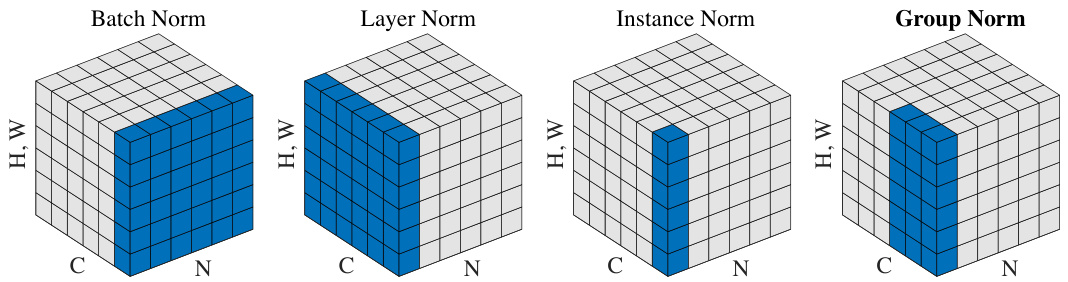
Figure 2. Normalization methods. Each subplot shows a feature map tensor, with $N$ as the batch axis, $C$ as the channel axis, and $(H,W)$ as the spatial axes. The pixels in blue are normalized by the same mean and variance, computed by aggregating the values of these pixels.
图 2: 归一化方法。每个子图展示了一个特征映射张量,其中 $N$ 为批次轴,$C$ 为通道轴,$(H,W)$ 为空间轴。蓝色像素通过相同的均值和方差进行归一化,这些值通过聚合这些像素的值计算得出。
3. Group Normalization
3. 组归一化
The channels of visual representations are not entirely independent. Classical features of SIFT [39], HOG [9], and GIST [41] are group-wise representations by design, where each group of channels is constructed by some kind of histogram. These features are often processed by groupwise normalization over each histogram or each orientation. Higher-level features such as VLAD [29] and Fisher Vectors (FV) [44] are also group-wise features where a group can be thought of as the sub-vector computed with respect to a cluster.
视觉表征的通道并非完全独立。SIFT [39]、HOG [9] 和 GIST [41] 的经典特征在设计上属于分组表征,每组通道通过某种直方图构建而成。这些特征通常通过针对每个直方图或方向的组归一化进行处理。更高层次的特征如 VLAD [29] 和 Fisher 向量 (FV) [44] 同样属于分组特征,其中每组可视为基于聚类计算的子向量。
Analogously, it is not necessary to think of deep neural network features as unstructured vectors. For example, for $\mathrm{conv_{1}}$ (the first convolutional layer) of a network, it is reasonable to expect a filter and its horizontal flipping to exhibit similar distributions of filter responses on natural images. If $\mathrm{conv_{1}}$ happens to approximately learn this pair of filters, or if the horizontal flipping (or other transformations) is made into the architectures by design [11, 8], then the corresponding channels of these filters can be normalized together.
类似地,我们不必将深度神经网络的特征视为非结构化向量。例如,对于网络的 $\mathrm{conv_{1}}$ (第一层卷积层),可以合理地预期一个滤波器及其水平翻转在自然图像上会表现出相似的滤波器响应分布。如果 $\mathrm{conv_{1}}$ 恰好近似学习了这对滤波器,或者通过设计将水平翻转(或其他变换)纳入架构 [11, 8],那么这些滤波器的对应通道就可以一起进行归一化。
The higher-level layers are more abstract and their behaviors are not as intuitive. However, in addition to orientations (SIFT [39], HOG [9], or [11, 8]), there are many factors that could lead to grouping, e.g., frequency, shapes, illumination, textures. Their coefficients can be interdependent. In fact, a well-accepted computational model in neuroscience is to normalize across the cell responses [21, 52, 55, 5], “with various receptive-field centers (covering the visual field) and with various s patio temporal frequency tunings” (p183, [21]); this can happen not only in the primary visual cortex, but also “throughout the visual system” [5]. Motivated by these works, we propose new generic group-wise normalization for deep neural networks.
高层级的特征更为抽象,其行为表现也较不直观。除方向特征(SIFT [39]、HOG [9]或[11, 8])外,频率、形状、光照、纹理等多种因素都可能引发特征分组,且这些特征的系数可能存在相互依赖关系。事实上,神经科学领域广为接受的计算模型是对细胞响应进行归一化处理[21, 52, 55, 5],即"通过具有不同感受野中心(覆盖视野范围)和不同空时频率调谐特性的细胞"(p183, [21])来实现——这种现象不仅存在于初级视觉皮层,还贯穿于"整个视觉系统"[5]。受这些研究启发,我们针对深度神经网络提出了一种新型通用分组归一化方法。
3.1. Formulation
3.1. 公式化
We first describe a general formulation of feature normalization, and then present GN in this formulation. A family of feature normalization methods, including BN, LN, IN, and GN, perform the following computation:
我们首先描述特征归一化的一般公式,然后在该框架下介绍GN。包括BN、LN、IN和GN在内的一系列特征归一化方法都执行以下计算:
$$
\hat{x}_ {i}=\frac{1}{\sigma_{i}}(x_{i}-\mu_{i}).
$$
$$
\hat{x}_ {i}=\frac{1}{\sigma_{i}}(x_{i}-\mu_{i}).
$$
Here $x$ is the feature computed by a layer, and $i$ is an index. In the case of 2D images, $i=(i_{N},i_{C},i_{H},i_{W})$ is a 4D vector indexing the features in $(N,C,H,W)$ order, where $N$ is the batch axis, $C$ is the channel axis, and $H$ and $W$ are the spatial height and width axes.
这里 $x$ 是由某层计算得到的特征,$i$ 是索引。对于二维图像,$i=(i_{N},i_{C},i_{H},i_{W})$ 是一个按 $(N,C,H,W)$ 顺序索引特征的4维向量,其中 $N$ 是批次轴,$C$ 是通道轴,$H$ 和 $W$ 分别是空间高度和宽度轴。
$\mu$ and $\sigma$ in (1) are the mean and standard deviation (std) computed by:
式(1)中的$\mu$和$\sigma$是通过以下公式计算得到的均值和标准差(std):
$$
\mu_{i}=\frac{1}{m}\sum_{k\in S_{i}}x_{k},\quad\sigma_{i}=\sqrt{\frac{1}{m}\sum_{k\in S_{i}}(x_{k}-\mu_{i})^{2}+\epsilon},
$$
$$
\mu_{i}=\frac{1}{m}\sum_{k\in S_{i}}x_{k},\quad\sigma_{i}=\sqrt{\frac{1}{m}\sum_{k\in S_{i}}(x_{k}-\mu_{i})^{2}+\epsilon},
$$
with $\epsilon$ as a small constant. $S_{i}$ is the set of pixels in which the mean and std are computed, and $m$ is the size of this set. Many types of feature normalization methods mainly differ in how the set $S_{i}$ is defined (Figure 2), discussed as follows.
其中 $\epsilon$ 是一个小常数。$S_{i}$ 是计算均值和标准差的像素集合,$m$ 是该集合的大小。多种特征归一化方法的主要区别在于如何定义集合 $S_{i}$ (图 2),具体讨论如下。
In Batch Norm [26], the set $S_{i}$ is defined as:
在批归一化 (Batch Norm) [26] 中,集合 $S_{i}$ 定义为:
$$
S_{i}={k\mid k_{C}=i_{C}},
$$
$$
S_{i}={k\mid k_{C}=i_{C}},
$$
where $i_{C}$ (and $k_{C}$ ) denotes the sub-index of $i$ (and $k$ ) along the $C$ axis. This means that the pixels sharing the same channel index are normalized together, i.e., for each channel, BN computes $\mu$ and $\sigma$ along the $(N,H,W)$ axes. In Layer Norm [3], the set is:
其中 $i_{C}$ (和 $k_{C}$) 表示 $i$ (和 $k$) 沿 $C$ 轴的子索引。这意味着共享相同通道索引的像素会一起进行归一化,即对于每个通道,BN (Batch Normalization) 沿 $(N,H,W)$ 轴计算 $\mu$ 和 $\sigma$。在层归一化 (Layer Norm) [3] 中,集合为:
$$
S_{i}={k\mid k_{N}=i_{N}},
$$
$$
S_{i}={k\mid k_{N}=i_{N}},
$$
meaning that LN computes $\mu$ and $\sigma$ along the $(C,H,W)$ axes for each sample. In Instance Norm [61], the set is:
这意味着 LN (Layer Normalization) 会为每个样本沿着 $(C,H,W)$ 轴计算 $\mu$ 和 $\sigma$。而在 Instance Norm [61] 中,计算集合为:
$$
S_{i}={k\mid k_{N}=i_{N},k_{C}=i_{C}}.
$$
$$
S_{i}={k\mid k_{N}=i_{N},k_{C}=i_{C}}.
$$
meaning that IN computes $\mu$ and $\sigma$ along the $(H,W)$ axes for each sample and each channel. The relations among BN, LN, and IN are in Figure 2.
这意味着IN会沿着$(H,W)$轴为每个样本和每个通道计算$\mu$和$\sigma$。BN、LN和IN之间的关系如图2所示。
As in [26], all methods of BN, LN, and IN learn a perchannel linear transform to compensate for the possible lost of representational ability:
如[26]所述,BN、LN和IN的所有方法都学习每个通道的线性变换,以补偿可能损失的表示能力:
$$
y_{i}=\gamma\hat{x}_{i}+\beta,
$$
$$
y_{i}=\gamma\hat{x}_{i}+\beta,
$$
where $\gamma$ and $\beta$ are trainable scale and shift (indexed by $i_{C}$ in all case, which we omit for simplifying notations).
其中 $\gamma$ 和 $\beta$ 是可训练的缩放和偏移参数 (在所有情况下都由 $i_{C}$ 索引,为简化表示此处省略)。
Group Norm. Formally, a Group Norm layer computes $\mu$ and $\sigma$ in a set $S_{i}$ defined as:
组归一化 (Group Norm)。形式上,组归一化层在集合$S_{i}$中计算$\mu$和$\sigma$,其定义为:
$$
S_{i}={k\mid k_{N}=i_{N},\lfloor\frac{k_{C}}{C/G}\rfloor=\lfloor\frac{i_{C}}{C/G}\rfloor}.
$$
$$
S_{i}={k\mid k_{N}=i_{N},\lfloor\frac{k_{C}}{C/G}\rfloor=\lfloor\frac{i_{C}}{C/G}\rfloor}.
$$
Here $G$ is the number of groups, which is a pre-defined hyper-parameter $\mathit{\Delta}G=32$ by default). $C/G$ is the num-ber of channels per group. $\lfloor\cdot\rfloor$ is the floor operation, and $\begin{array}{r}{\dot{\bf\ L}\frac{k_{C}}{C/G}\bigr\rfloor=\frac{i_{C}}{C/G}\biggr\rfloor}\end{array}$ ” means that the indexes $i$ and $k$ are in the same group of channels, assuming each group of channels are stored in a sequential order along the $C$ axis. GN computes $\mu$ and $\sigma$ along the $(H,W)$ axes and along a group of $\frac{\dot{C}}{G}$ channels. The computation of GN is illustrated in Figure 2 (rightmost), which is a simple case of 2 groups G=2 ) each having 3 channels.
这里 $G$ 是组数,它是一个预定义的超参数(默认值为 $\mathit{\Delta}G=32$)。$C/G$ 是每组的通道数。$\lfloor\cdot\rfloor$ 是向下取整运算,而 $\begin{array}{r}{\dot{\bf\ L}\frac{k_{C}}{C/G}\bigr\rfloor=\frac{i_{C}}{C/G}\biggr\rfloor}\end{array}$ 表示索引 $i$ 和 $k$ 位于同一通道组中,假设每组通道沿 $C$ 轴按顺序存储。GN 沿着 $(H,W)$ 轴和一组 $\frac{\dot{C}}{G}$ 通道计算 $\mu$ 和 $\sigma$。GN 的计算如图 2(最右侧)所示,这是一个简单的情况,包含 2 组(G=2)通道,每组有 3 个通道。
Given $S_{i}$ in Eqn.(7), a GN layer is defined by Eqn.(1), (2), and (6). Specifically, the pixels in the same group are normalized together by the same $\mu$ and $\sigma$ . GN also learns the per-channel $\gamma$ and $\beta$ .
给定式 (7) 中的 $S_{i}$,GN (Group Normalization) 层由式 (1)、(2) 和 (6) 定义。具体而言,同一组内的像素通过相同的 $\mu$ 和 $\sigma$ 进行归一化。GN 还会学习每个通道的 $\gamma$ 和 $\beta$。
Relation to Prior Work. LN, IN, and GN all perform independent computations along the batch axis. The two extreme cases of GN are equivalent to LN and IN (Figure 2).
与先前工作的关系。层归一化 (LN) 、实例归一化 (IN) 和组归一化 (GN) 均沿批次轴执行独立计算。GN 的两种极端情况分别等价于 LN 和 IN (图 2)。
Relation to Layer Normalization [3]. GN becomes LN if we set the group number as $G=1$ . LN assumes all channels in a layer make “similar contributions” [3]. Unlike the case of fully-connected layers studied in [3], this assumption can be less valid with the presence of convolutions, as discussed in [3]. GN is less restricted than LN, because each group of channels (instead of all of them) are assumed to subject to the shared mean and variance; the model still has flexibility of learning a different distribution for each group. This leads to improved representational power of GN over LN, as shown by the lower training and validation error in experiments (Figure 4).
与层归一化 (Layer Normalization) [3] 的关系。若将组数设为 $G=1$ ,GN 即退化为 LN。LN 假设层中所有通道的"贡献相似" [3],但如 [3] 所述,当存在卷积操作时(与全连接层不同),这一假设可能不再成立。GN 的限制比 LN 更宽松,因为其仅要求每组通道(而非全部通道)共享均值和方差,模型仍可学习不同组的独立分布特性。如图 4 所示,这种特性使 GN 比 LN 具有更强的表征能力,表现为更低的训练误差和验证误差。
Relation to Instance Normalization [61]. GN becomes IN if we set the group number as $G=C$ (i.e., one channel per group). But IN can only rely on the spatial dimension for computing the mean and variance and it misses the opportunity of exploiting the channel dependence.
与实例归一化(Instance Normalization) [61]的关系。若将组数设为$G=C$(即每组一个通道),GN就退化为IN。但IN仅能依靠空间维度计算均值与方差,丧失了利用通道间依赖关系的机会。
3.2. Implementation
3.2. 实现
GN can be easily implemented by a few lines of code in PyTorch [42] and TensorFlow [1] where automatic differentiation is supported. Figure 3 shows the code based on
GN可以通过几行代码在支持自动微分的PyTorch [42]和TensorFlow [1]中轻松实现。图3展示了基于
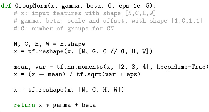
Figure 3. Python code of Group Norm based on TensorFlow.
图 3: 基于 TensorFlow 的 Group Norm 的 Python语言 代码。
TensorFlow. In fact, we only need to specify how the mean and variance (“moments”) are computed, along the appropriate axes as defined by the normalization method.
TensorFlow。实际上,我们只需指定均值和方差("矩")的计算方式,并按照归一化方法定义的适当轴进行计算。
4. Experiments
4. 实验
4.1. Image Classification in ImageNet
4.1. ImageNet 图像分类
We experiment in the ImageNet classification dataset [50] with 1000 classes. We train on the ${\sim}1.28\mathrm{M}$ training images and evaluate on the 50,000 validation images, using the ResNet models [20].
我们在ImageNet分类数据集[50]上进行了实验,该数据集包含1000个类别。我们使用ResNet模型[20]在约128万张训练图像上进行训练,并在5万张验证图像上评估模型性能。
Implementation details. As standard practice [20, 17], we use 8 GPUs to train all models, and the batch mean and variance of BN are computed within each GPU. We use the method of [19] to initialize all convolutions for all models. We use 1 to initialize all $\gamma$ parameters, except for each residual block’s last normalization layer where we initialize $\gamma$ by 0 following [16] (such that the initial state of a residual block is identity). We use a weight decay of 0.0001 for all weight layers, including $\gamma$ and $\beta$ (following [17] but unlike [20, 16]). We train 100 epochs for all models, and decrease the learning rate by $10\times$ at 30, 60, and 90 epochs. During training, we adopt the data augmentation of [58] as implemented by [17]. We evaluate the top-1 classification error on the center crops of $224\times224$ pixels in the validation set. To reduce random variations, we report the median error rate of the final 5 epochs [16]. Other implementation details follow [17].
实现细节。按照标准做法 [20, 17],我们使用8块GPU训练所有模型,并在每个GPU内计算BN的批次均值和方差。我们采用[19]的方法初始化所有模型的卷积层。除残差块最后一个归一化层的$\gamma$参数按[16]初始化为0(使残差块的初始状态为恒等变换)外,其余$\gamma$参数均初始化为1。所有权重层(包括$\gamma$和$\beta$)的权重衰减设为0.0001(遵循[17]但不同于[20, 16])。所有模型训练100个周期,学习率在第30、60、90周期时下降$10\times$。训练中采用[17]实现的[58]数据增强方法。我们在验证集上评估$224\times224$像素中心裁剪的top-1分类错误率。为减少随机波动,报告最后5个周期的错误率中位数[16]。其他实现细节遵循[17]。
Our baseline is the ResNet trained with BN [20]. To compare with LN, IN, and GN, we replace BN with the specific variant. We use the same hyper-parameters for all models. We set $G=32$ for GN by default.
我们的基线是使用BN [20]训练的ResNet。为了与LN、IN和GN进行比较,我们用特定变体替换了BN。所有模型使用相同的超参数。默认情况下,我们将GN的$G=32$。
Comparison of feature normalization methods. We first experiment with a regular batch size of 32 images (per GPU) [26, 20]. BN works successfully in this regime, so this is a strong baseline to compare with. Figure 4 shows the error curves, and Table 1 shows the final results.
特征归一化方法对比。我们首先在每GPU 32张图像的常规批量大小下进行实验 [26, 20]。BN (Batch Normalization) 在该场景下表现良好,因此这是一个强有力的对比基线。图4展示了错误率曲线,表1列出了最终结果。
Figure 4 shows that all of these normalization methods are able to converge. LN has a small degradation of $1.7%$ comparing with BN. This is an encouraging result, as it suggests that normalizing along all channels (as done by LN) of a convolutional network is reasonably good. IN also makes the model converge, but is $4.8%$ worse than BN.3
图 4 显示所有这些归一化方法都能收敛。LN (Layer Normalization) 相比 BN (Batch Normalization) 仅有 1.7% 的小幅性能下降。这一结果令人鼓舞,表明在卷积网络中沿所有通道进行归一化(如LN所做)的效果相当不错。IN (Instance Normalization) 也能使模型收敛,但性能比 BN 低 4.8%。[3]
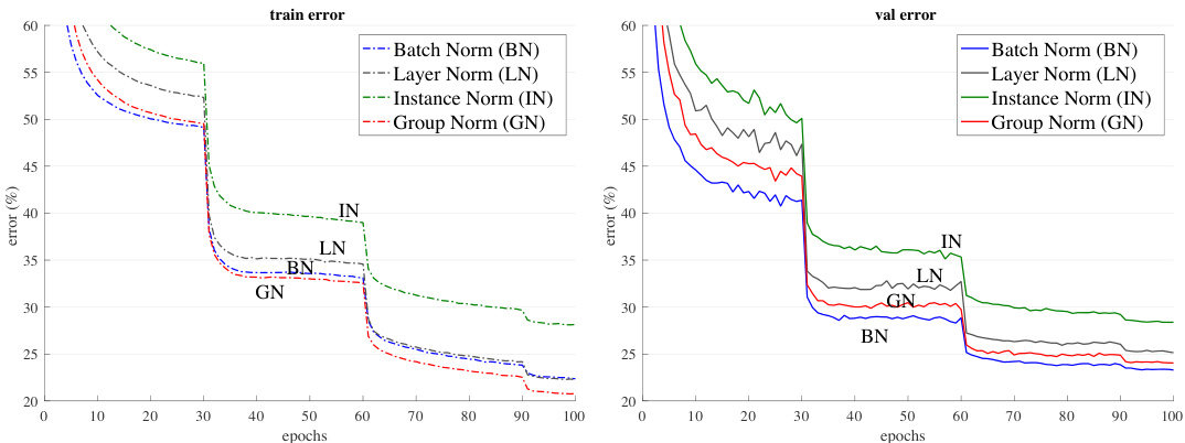
Figure 4. Comparison of error curves with a batch size of 32 images/GPU. We show the ImageNet training error (left) and validation error (right) vs. numbers of training epochs. The model is ResNet-50.
图 4: 批大小为32张图像/GPU时的误差曲线对比。我们展示了ImageNet训练误差(左)和验证误差(右)随训练周期数的变化情况。模型为ResNet-50。
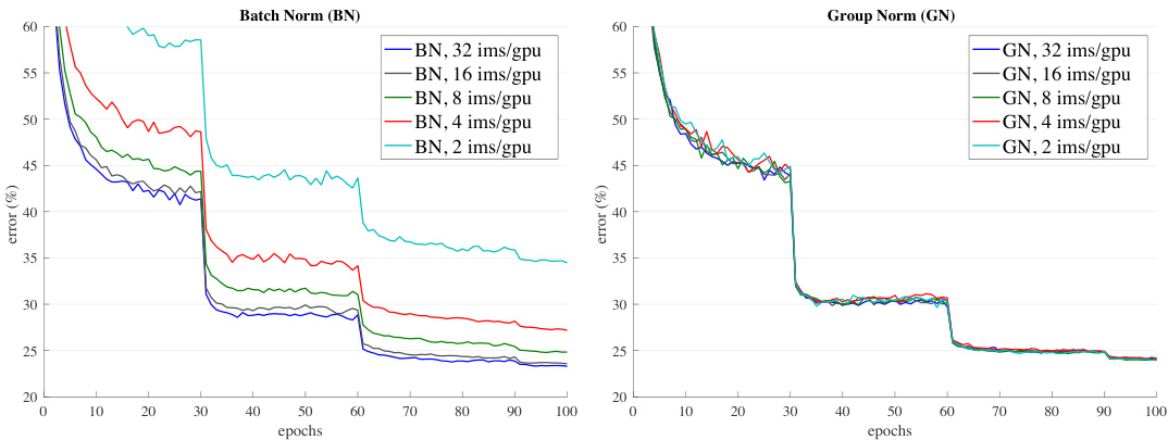
Figure 5. Sensitivity to batch sizes: ResNet-50’s validation error of BN (left) and GN (right) trained with 32, 16, 8, 4, and 2 images/GPU.
图 5: 批量大小敏感性:使用每GPU 32、16、8、4和2张图像训练的BN(左)和GN(右)的ResNet-50验证误差。
Table 1. Comparison of error rates $(%)$ of ResNet-50 in the ImageNet validation set, trained with a batch size of 32 images/GPU. The error curves are in Figure 4.
| BN | LN | IN | GN | |
| val error | 23.6 | 25.3 | 28.4 | 24.1 |
| △ (vs. BN) | 1.7 | 4.8 | 0.5 |
表 1: ResNet-50在ImageNet验证集上的错误率 $(%)$ 对比,批大小为32张图像/GPU。错误曲线见图4。
| BN | LN | IN | GN | |
|---|---|---|---|---|
| val error | 23.6 | 25.3 | 28.4 | 24.1 |
| △ (vs. BN) | 1.7 | 4.8 | 0.5 |
In this regime where BN works well, GN is able to approach BN’s accuracy, with a decent degradation of $0.5%$ in the validation set. Actually, Figure 4 (left) shows that GN has lower training error than BN, indicating that GN is effective for easing optimization. The slightly higher validation error of GN implies that GN loses some regular iz ation ability of BN. This is understandable, because BN’s mean and variance computation introduces uncertainty caused by the stochastic batch sampling, which helps regular iz ation [26]. This uncertainty is missing in GN (and LN/IN). But it is possible that GN combined with a suitable regularize r will improve results. This can be a future research topic.
在这一BN表现良好的情况下,GN能够接近BN的准确率,验证集上仅有0.5%的适度性能下降。实际上,图4(左)显示GN的训练误差低于BN,表明GN能有效缓解优化难题。GN略高的验证误差意味着其损失了BN的部分正则化能力。这可以理解,因为BN通过随机批量采样计算均值方差引入的不确定性有助于正则化[26],而GN(及LN/IN)缺乏这种不确定性。但GN配合合适的正则化器可能提升效果,这值得未来研究。
Table 2. Sensitivity to batch sizes. We show ResNet-50’s validation error $(%)$ in ImageNet. The last row shows the differences between BN and GN. The error curves are in Figure 5. This table is visualized in Figure 1.
| batch size | 32 | 16 | 8 | 4 | 2 |
| BN | 23.6 | 23.7 | 24.8 | 27.3 | 34.7 |
| GN | 24.1 | 24.2 | 24.0 | 24.2 | 24.1 |
| △ | 0.5 | 0.5 | -0.8 | -3.1 | -10.6 |
表 2: 批量大小的敏感性。我们展示了ResNet-50在ImageNet上的验证错误率 $(%)$ 。最后一行显示了BN (Batch Normalization) 和GN (Group Normalization) 之间的差异。错误曲线见图 5。本表可视化结果见图 1。
| 批量大小 | 32 | 16 | 8 | 4 | 2 |
|---|---|---|---|---|---|
| BN | 23.6 | 23.7 | 24.8 | 27.3 | 34.7 |
| GN | 24.1 | 24.2 | 24.0 | 24.2 | 24.1 |
| △ | 0.5 | 0.5 | -0.8 | -3.1 | -10.6 |
Small batch sizes. Although BN benefits from the stochasticity under some situations, its error increases when the batch size becomes smaller and the uncertainty gets bigger. We show this in Figure 1, Figure 5, and Table 2.
小批量大小。尽管BN在某些情况下受益于随机性,但当批量变小时其误差会增大,不确定性也随之增加。我们在图1、图5和表2中展示了这一现象。
We evaluate batch sizes of 32, 16, 8, 4, 2 images per GPU. In all cases, the BN mean and variance are computed within each GPU and not synchronized. All models are trained in 8 GPUs. In this set of experiments, we adopt the linear learning rate scaling rule [31, 4, 16] to adapt to batch size changes — we use a learning rate of 0.1 [20] for the batch size of 32, and $0.1N/32$ for a batch size of $N$ . This linear scaling rule works well for BN if the total batch size changes (by changing the number of GPUs) but the perGPU batch size does not change [16]. We keep the same number of training epochs for all cases (Figure 5, $\mathbf{X}$ -axis). All other hyper-parameters are unchanged.
我们评估了每块GPU处理32、16、8、4、2张图像的批次大小。在所有情况下,批量归一化(BN)的均值和方差都在每块GPU内部计算且不进行同步。所有模型均在8块GPU上训练。本组实验中,我们采用线性学习率缩放规则[31,4,16]来适应批次大小变化——当批次大小为32时使用0.1的学习率[20],批次大小为$N$时使用$0.1N/32$。该线性缩放规则在总批次大小变化(通过改变GPU数量)而单GPU批次大小不变时对BN效果良好[16]。所有情况下保持相同训练周期数(图5 $\mathbf{X}$轴),其余超参数保持不变。
| error | |
| none | 29.2 |
| BN GN | 28.0 27.6 |
| error | |
|---|---|
| none | 29.2 |
| BN GN | 28.0 27.6 |
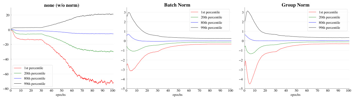
Figure 6. Evolution of feature distributions of $\mathrm{conv_{5,3}}$ ’s output (before normalization and ReLU) from VGG-16, shown as the {1,20,80,99} percentile of responses. The table on the right shows the ImageNet validation error $(%)$ . Models are trained with 32 images/GPU.
图 6: VGG-16中$\mathrm{conv_{5,3}}$输出(归一化和ReLU前)的特征分布演变,以响应值的{1,20,80,99}百分位表示。右侧表格显示ImageNet验证错误率$(%)$。模型训练使用32张图像/GPU。
| # groups (G) | |||||||
| 64 | 32 | 16 | 8 | 4 | 2 | 1 (=LN) | |
| 24.6 0.5 | 24.1 | 24.6 0.5 | 24.4 0.3 | 24.6 0.5 | 24.7 0.6 | 25.3 1.2 | |
| # channels per group | |||||||
| 64 | 32 | 16 | 8 | 4 | 2 | 1 (=IN) | |
| 24.4 | 24.5 | 24.2 | 24.3 | 24.8 | 25.6 | 28.4 | |
| 0.2 | 0.3 | 0.1 | 0.6 | 1.4 | 4.2 | ||
| # 组数 (G) | 64 | 32 | 16 | 8 | 4 | 2 | 1 (=LN) |
|---|---|---|---|---|---|---|---|
| 24.6 ±0.5 | 24.1 | 24.6 ±0.5 | 24.4 ±0.3 | 24.6 ±0.5 | 24.7 ±0.6 | 25.3 ±1.2 |
| 每组通道数 | 64 | 32 | 16 | 8 | 4 | 2 | 1 (=IN) |
|---|---|---|---|---|---|---|---|
| 24.4 | 24.5 | 24.2 | 24.3 | 24.8 | 25.6 | 28.4 | |
| ±0.2 | ±0.3 | ±0.1 | ±0.6 | ±1.4 | ±4.2 |
Table 3. Group division. We show ResNet-50’s validation error $(%)$ in ImageNet, trained with 32 images/GPU. (Top): a given number of groups. (Bottom): a given number of channels per group. The last rows show the differences with the best number.
表 3: 分组划分。我们展示了在 ImageNet 上训练的 ResNet-50 验证错误率 $(%)$ (32 张图像/GPU)。 (上): 给定组数。 (下): 给定每组通道数。最后一行显示与最佳数值的差异。
Figure 5 (left) shows that BN’s error becomes considerably higher with small batch sizes. GN’s behavior is more stable and insensitive to the batch size. Actually, Figure 5 (right) shows that GN has very similar curves (subject to random variations) across a wide range of batch sizes from 32 to 2. In the case of a batch size of 2, GN has $10.6%$ lower error rate than its BN counterpart $(24.1%\nu s.34.7%)$ .
图 5 (左) 显示 BN 的误差在小批量大小时显著增加。GN 的表现更为稳定,对批量大小不敏感。实际上,图 5 (右) 表明 GN 在批量大小从 32 到 2 的广泛范围内具有非常相似的曲线(存在随机波动)。当批量大小为 2 时,GN 的误差率比 BN 低 10.6% (24.1% vs. 34.7%)。
These results indicate that the batch mean and variance estimation can be overly stochastic and inaccurate, especially when they are computed over 4 or 2 images. However, this stochastic it y disappears if the statistics are computed from 1 image, in which case BN becomes similar to IN at training time. We see that IN has a better result $(28.4%)$ than BN with a batch size of 2 $(34.7%)$ .
这些结果表明,批量均值和方差估计可能过于随机且不准确,尤其是在基于4张或2张图像计算时。然而,若统计量仅从单张图像计算,这种随机性就会消失,此时批量归一化 (BN) 在训练时会变得类似于实例归一化 (IN)。数据显示,当批量大小为2时,IN的表现 $(28.4%)$ 优于BN $(34.7%)$。
The robust results of GN in Table 2 demonstrate GN’s strength. It allows to remove the batch size constraint imposed by BN, which can give considerably more memory (e.g., $16\times$ or more). This will make it possible to train higher-capacity models that would be otherwise bottlenecked by memory limitation. We hope this will create new opportunities in architecture design.
表 2 中 GN 的稳健结果证明了 GN 的优势。它能够消除 BN 对批处理大小的限制,从而显著提升内存利用率 (例如 $16\times$ 或更高)。这将使得训练更高容量的模型成为可能,而这些模型原本会受限于内存瓶颈。我们希望这能为架构设计带来新的机遇。
Comparison with Batch Renorm (BR). BR [25] introduces two extra parameters $(r$ and $d$ in [25]) that constrain the estimated mean and variance of BN. Their values are controlled by $r_{\mathrm{max}}$ and $d_{\mathrm{max}}$ . To apply BR to ResNet-50, we have carefully chosen these hyper-parameters, and found that $r_{\operatorname*{max}}=1.5$ and $d_{\operatorname*{max}}=0.5$ work best for ResNet-50.
与批量重归一化(BR)的对比。BR [25]引入了两个额外参数$(r$和$d$[25])来约束BN的估计均值和方差。这些参数值由$r_{\mathrm{max}}$和$d_{\mathrm{max}}$控制。为将BR应用于ResNet-50,我们精心选择了这些超参数,发现$r_{\operatorname*{max}}=1.5$和$d_{\operatorname*{max}}=0.5$在ResNet-50上表现最佳。
With a batch size of 4, ResNet-50 trained with BR has an error rate of $26.3%$ . This is better than BN’s $27.3%$ , but still $2.1%$ higher than GN’s $24.2%$ .
在批大小为4时,使用BR训练的ResNet-50错误率为$26.3%$。这优于BN的$27.3%$,但仍比GN的$24.2%$高出$2.1%$。
Group division. Thus far all presented GN models are trained with a group number of $G=32$ . Next we evaluate different ways of dividing into groups. With a given fixed group number, GN performs reasonably well for all values of $G$ we studied (Table 3, top panel). In the extreme case of $G=1$ , GN is equivalent to LN, and its error rate is higher than all cases of $G>1$ studied.
分组划分。目前为止,所有展示的GN模型均采用分组数$G=32$进行训练。接下来我们评估不同的分组方式。在给定固定分组数的情况下,GN在我们研究的所有$G$值下都表现良好(表3,上半部分)。在极端情况$G=1$时,GN等价于LN,其错误率高于我们研究的所有$G>1$情况。
We also evaluate fixing the number of channels per group (Table 3, bottom panel). Note that because the layers can have different channel numbers, the group number $G$ can change across layers in this setting. In the extreme case of 1 channel per group, GN is equivalent to IN. Even if using as few as 2 channels per group, GN has substantially lower error than IN $25.6%$ vs. $28.4%$ ). This result shows the effect of grouping channels when performing normalization.
我们还评估了固定每组通道数的情况(表3, 底部面板)。需要注意的是, 由于各层可能具有不同的通道数, 在这种设置下组数$G$会随层而变化。在每组1个通道的极端情况下, GN (Group Normalization)等同于IN (Instance Normalization)。即使每组仅使用2个通道, GN的错误率也显著低于IN ($25.6%$ vs. $28.4%$)。这一结果表明了在执行归一化时对通道进行分组的效果。
Deeper models. We have also compared GN with BN on ResNet-101 [20]. With a batch size of 32, our BN baseline of ResNet-101 has $22.0%$ validation error, and the GN counterpart has $22.4%$ , slightly worse by $0.4%$ . With a batch size of 2, GN ResNet-101’s error is $23.0%$ . This is still a decently stable result considering the very small batch size, and it is $8.9%$ better than the BN counterpart’s $31.9%$ .
更深的模型。我们还在ResNet-101 [20]上比较了GN与BN。当批量大小为32时,我们的BN基线ResNet-101验证错误率为$22.0%$,而GN版本为$22.4%$,稍差$0.4%$。当批量大小为2时,GN ResNet-101的错误率为$23.0%$。考虑到极小的批量大小,这仍然是一个相当稳定的结果,并且比BN版本的$31.9%$高出$8.9%$。
Results and analysis of VGG models. To study GN/BN compared to no normalization, we consider VGG-16 [56] that can be healthily trained without normalization layers. We apply BN or GN right after each convolutional layer. Figure 6 shows the evolution of the feature distributions of $\mathrm{conv_{5,3}}$ (the last convolutional layer). GN and BN behave qualitatively similar, while being substantially different with the variant that uses no normalization; this phenomenon is also observed for all other convolutional layers. This comparison suggests that performing normalization is essential for controlling the distribution of features.
VGG模型的实验结果与分析。为了研究GN/BN与无归一化处理的对比,我们选用无需归一化层也能正常训练的VGG-16[56]架构,在每个卷积层后立即应用BN或GN。图6展示了$\mathrm{conv_{5,3}}$(最后一层卷积层)特征分布的演变过程:GN与BN在性质上表现相似,但与未使用归一化的变体存在显著差异,该现象在其他所有卷积层中同样存在。这一对比表明,执行归一化处理对于控制特征分布至关重要。
For VGG-16, GN is better than BN by $0.4%$ (Figure 6, right). This possibly implies that VGG-16 benefits less from BN’s regular iz ation effect, and GN (that leads to lower training error) is superior to BN in this case.
对于VGG-16,GN (Group Normalization) 比BN (Batch Normalization) 高出$0.4%$ (图6右)。这可能意味着VGG-16从BN的正则化效果中获益较少,而GN (能带来更低的训练误差) 在这种情况下优于BN。
4.2. Object Detection and Segmentation in COCO
4.2. COCO 数据集中的目标检测与分割
Next we evaluate fine-tuning the models for transferring to object detection and segmentation. These computer vision tasks in general benefit from higher-resolution input, so the batch size tends to be small in common practice (1 or 2 images/GPU [12, 47, 18, 36]). As a result, BN is turned into a linear layer $\begin{array}{r}{y=\frac{\gamma}{\sigma}(x-\mu)+\beta}\end{array}$ where $\mu$ and $\sigma$ are pre-computed from the pre-trained model and frozen [20]. We denote this as $\mathbf{BN}^{*}$ , which in fact performs no normalization during fine-tuning. We have also tried a variant that fine-tunes BN (normalization is performed and not frozen) and found it works poorly (reducing ${\sim}6$ AP with a batch size of 2), so we ignore this variant.
接下来我们评估模型在目标检测和分割任务上的微调效果。这些计算机视觉任务通常受益于更高分辨率的输入,因此实际应用中批量大小往往较小(1或2张图像/GPU [12, 47, 18, 36])。因此,批归一化(BN)被转化为线性层 $\begin{array}{r}{y=\frac{\gamma}{\sigma}(x-\mu)+\beta}\end{array}$ ,其中 $\mu$ 和 $\sigma$ 是从预训练模型中预计算并冻结的参数 [20]。我们将此记为 $\mathbf{BN}^{*}$ ,实际上在微调过程中不执行归一化操作。我们还尝试了微调BN的变体(执行归一化且不冻结参数),发现效果较差(批量大小为2时AP下降约6点),因此不再考虑该变体。
We experiment on the Mask R-CNN baselines [18], implemented in the publicly available codebase of Detectron [13]. We use the end-to-end variant with the same hyperparameters as in [13]. We replace $\mathbf{BN}^{*}$ with GN during finetuning, using the corresponding models pre-trained from ImageNet.4 During fine-tuning, we use a weight decay of 0 for the $\gamma$ and $\beta$ parameters, which is important for good detection results when $\gamma$ and $\beta$ are being tuned. We fine-tune with a batch size of 1 image/GPU and 8 GPUs.
我们在Mask R-CNN基线模型[18]上进行实验,该模型基于公开的Detectron代码库[13]实现。我们采用与[13]相同的超参数设置进行端到端变体训练。在微调阶段,我们将$\mathbf{BN}^{*}$替换为GN (Group Normalization),并使用对应的ImageNet预训练模型。微调时,我们对$\gamma$和$\beta$参数采用0权重衰减策略——当需要调整$\gamma$和$\beta$时,这对获得良好检测结果至关重要。实验使用8块GPU,每GPU处理1张图像的批量大小进行微调。
The models are trained in the COCO train2017 set and evaluated in the COCO val2017 set (a.k.a minival). We report the standard COCO metrics of Average Precision (AP), $\mathrm{AP}_ {50}$ , and $\mathrm{AP}_{75}$ , for bounding box detection $(\mathrm{AP^{bbox}})$ ) and instance segmentation $(\mathbf{AP}^{\mathrm{mask}})$ .
模型在COCO train2017数据集上训练,并在COCO val2017数据集(又称minival)上评估。我们报告了标准COCO指标:平均精度(AP)、$\mathrm{AP}_ {50}$和$\mathrm{AP}_{75}$,分别用于边界框检测$(\mathrm{AP^{bbox}})$和实例分割$(\mathbf{AP}^{\mathrm{mask}})$。
Results of C4 backbone. Table 4 shows the comparison of GN vs. $\mathbf{BN}^{*}$ on Mask R-CNN using a $\mathrm{conv_{4}}$ backbone $(^{66}{\mathrm{C}}4^{,})$ [18]). This C4 variant uses ResNet’s layers of up to $\mathrm{conv_{4}}$ to extract feature maps, and ResNet’s $\mathrm{conv}_{5}$ layers as the Region-of-Interest (RoI) heads for classification and regression. As they are inherited from the pre-trained model, the backbone and head both involve normalization layers.
C4主干网络的结果。表4展示了在Mask R-CNN上使用$\mathrm{conv_{4}}$主干网络$(^{66}{\mathrm{C}}4^{,})$[18]时,GN与$\mathbf{BN}^{*}$的比较。这个C4变体使用ResNet的$\mathrm{conv_{4}}$及以下层来提取特征图,并将ResNet的$\mathrm{conv}_{5}$层作为分类和回归的感兴趣区域(RoI)头部。由于它们继承自预训练模型,主干网络和头部都包含归一化层。
On this baseline, GN improves over $\mathbf{BN}^{ * }$ by 1.1 box AP and 0.8 mask AP. We note that the pre-trained GN model is slightly worse than BN in ImageNet $24.1%$ vs. $23.6%$ ), but GN still outperforms $\mathbf{BN}^{ * }$ for fine-tuning. $\mathbf{BN}^{*}$ creates inconsistency between pre-training and fine-tuning (frozen), which may explain the degradation.
在此基线基础上,GN比$\mathbf{BN}^{ * }$提升了1.1个框AP和0.8个掩码AP。我们注意到预训练的GN模型在ImageNet上略逊于BN ($24.1%$ vs. $23.6%$),但GN在微调阶段仍优于$\mathbf{BN}^{ * }$。$\mathbf{BN}^{*}$导致预训练与(冻结状态)微调之间的不一致性,这可能是性能下降的原因。
We have also experimented with the LN variant, and found it is 1.9 box AP worse than GN and 0.8 worse than $\mathbf{BN}^{*}$ . Although LN is also independent of batch sizes, its representational power is weaker than GN.
我们还测试了LN变体,发现其性能比GN低1.9个框AP (average precision) ,比$\mathbf{BN}^{*}$低0.8。尽管LN同样不受批量大小影响,但其表征能力弱于GN。
Results of FPN backbone. Next we compare GN and $\mathbf{BN}^{*}$ on Mask R-CNN using a Feature Pyramid Network (FPN) backbone [35], the currently state-of-the-art framework in COCO. Unlike the C4 variant, FPN exploits all pre-trained layers to construct a pyramid, and appends randomly initialized layers as the head. In [35], the box head consists of two hidden fully-connected layers (2fc). We find that replacing the 2fc box head with 4conv1fc (similar to [48]) can better leverage GN. The resulting comparisons are in Table 5.
FPN主干网络的实验结果。接下来我们比较了在Mask R-CNN中使用特征金字塔网络(FPN)主干[35]时GN和$\mathbf{BN}^{*}$的表现,这是当前COCO数据集上最先进的框架。与C4变体不同,FPN利用所有预训练层构建金字塔结构,并添加随机初始化的层作为头部。在[35]中,边界框头部由两个全连接隐藏层(2fc)组成。我们发现将2fc边界框头部替换为4conv1fc(类似[48])能更好地发挥GN的优势。最终比较结果如表5所示。
Table 4. Detection and segmentation ablation results in COCO, using Mask R-CNN with ResNet-50 C4. $\mathbf{BN}^{*}$ means BN is frozen.
| backbone | Apbbox | APbox | APbbox | Apmask | ||
| BN* | 37.7 | 57.9 | 40.9 | 32.8 | 54.3 | 34.7 |
| GN | 38.8 | 59.2 | 42.2 | 33.6 | 55.9 | 35.4 |
表 4: 使用 ResNet-50 C4 的 Mask R-CNN 在 COCO 上的检测和分割消融实验结果。$\mathbf{BN}^{*}$ 表示 BN 被冻结。
| backbone | Apbbox | APbox | APbbox | Apmask | ||
|---|---|---|---|---|---|---|
| BN* | 37.7 | 57.9 | 40.9 | 32.8 | 54.3 | 34.7 |
| GN | 38.8 | 59.2 | 42.2 | 33.6 | 55.9 | 35.4 |
Table 5. Detection and segmentation ablation results in COCO, using Mask R-CNN with ResNet-50 FPN and a 4conv1fc bounding box head. $\mathbf{BN}^{*}$ means BN is frozen.
| backbone | boxhead | APbbox | APbbox | APbbox | APmask | APmask | APmask |
| BN* | 38.6 | 59.5 | 41.9 | 34.2 | 56.2 | 36.1 | |
| BN* | GN | 39.5 | 60.0 | 43.2 | 34.4 | 56.4 | 36.3 |
| GN | GN | 40.0 | 61.0 | 43.3 | 34.8 | 57.3 | 36.3 |
表 5: 在COCO数据集上使用Mask R-CNN (ResNet-50 FPN骨干网络和4conv1fc边界框头) 的检测与分割消融实验结果。$\mathbf{BN}^{*}$ 表示冻结BN层。
| backbone | boxhead | APbbox | APbbox | APbbox | APmask | APmask | APmask |
|---|---|---|---|---|---|---|---|
| BN* | 38.6 | 59.5 | 41.9 | 34.2 | 56.2 | 36.1 | |
| BN* | GN | 39.5 | 60.0 | 43.2 | 34.4 | 56.4 | 36.3 |
| GN | GN | 40.0 | 61.0 | 43.3 | 34.8 | 57.3 | 36.3 |
| Apbbox APbbox 50 | APbbox 75 | Apmask | APmask 50 | Apmask 75 | |
| R50BN R50 GN R50 GN, long | 38.6 59.8 40.3 61.0 40.8 61.6 | 42.1 44.0 44.4 | 34.5 35.7 36.1 | 56.4 57.9 | 36.3 37.7 38.2 |
| R101 BN R101 GN | 40.9 41.8 | 61.9 44.8 62.5 45.4 | 36.4 36.8 | 58.5 58.5 59.2 | 38.7 39.0 |
Table 6. Detection and segmentation results in COCO using Mask R-CNN and FPN. Here $\mathbf{BN}^{*}$ is the default Detectron baseline [13], and GN is applied to the backbone, box head, and mask head. “long” means training with more iterations. Code of these results are in https://github.com/facebook research/ Detectron/blob/master/projects/GN.
| Apbbox APbbox 50 | APbbox 75 | Apmask | APmask 50 | Apmask 75 | |
|---|---|---|---|---|---|
| R50BN R50 GN R50 GN, long | 38.6 59.8 40.3 61.0 40.8 61.6 | 42.1 44.0 44.4 | 34.5 35.7 36.1 | 56.4 57.9 | 36.3 37.7 38.2 |
| R101 BN R101 GN | 40.9 41.8 | 61.9 44.8 62.5 45.4 | 36.4 36.8 | 58.5 58.5 59.2 | 38.7 39.0 |
表 6: 使用Mask R-CNN和FPN在COCO数据集上的检测与分割结果。其中$\mathbf{BN}^{*}$是默认的Detectron基线[13],GN被应用于骨干网络、检测头和分割头。"long"表示更长时间的训练迭代。相关代码见https://github.com/facebookresearch/Detectron/blob/master/projects/GN。
As a baseline, $\mathbf{BN}^{ * }$ has 38.6 box AP using the 4conv1fc head, on par with its 2fc counterpart using the same pretrained model (38.5 AP). By adding GN to all convolutional layers of the box head (but still using the $\mathbf{BN}^{*}$ backbone), we increase the box AP by 0.9 to 39.5 (2nd row, Table 5). This ablation shows that a substantial portion of GN’s improvement for detection is from normalization in the head (which is also done by the C4 variant). On the contrary, applying BN to the box head (that has 512 RoIs per image) does not provide satisfactory result and is ${\sim}9$ AP worse — in detection, the batch of RoIs are sampled from the same image and their distribution is not i.i.d., and the non-i.i.d. distribution is also an issue that degrades BN’s batch statistics estimation [25]. GN does not suffer from this problem.
作为基线,$\mathbf{BN}^{ * }$在使用4conv1fc头时达到38.6的框AP (box AP) ,与使用相同预训练模型的2fc对应版本(38.5 AP)相当。通过在框头的所有卷积层添加GN (但主干仍使用$\mathbf{BN}^{*}$) ,我们将框AP提高了0.9至39.5 (表5第2行) 。该消融实验表明,GN在检测中的大部分改进来自头部的归一化 (C4变体也采用了这种方式) 。相反,对框头 (每张图像有512个RoI) 应用BN无法获得理想结果,其AP值低约9——在检测中,RoI批次是从同一图像采样的,其分布不具备独立同分布特性,这种非独立同分布问题也会影响BN的批次统计量估计[25]。GN则不受此问题影响。
Next we replace the FPN backbone with the GN-based counterpart, i.e., the GN pre-trained model is used during fine-tuning (3rd row, Table 5). Applying GN to the backbone alone contributes a $0.5~\mathrm{AP}$ gain (from 39.5 to 40.0), suggesting that GN helps when transferring features.
接下来我们将FPN主干网络替换为基于GN (Group Normalization) 的对应版本,即在微调阶段使用GN预训练模型 (表5第3行)。仅对主干网络应用GN就带来了0.5 AP的性能提升 (从39.5提高到40.0),这表明GN有助于特征迁移。

Figure 7. Error curves in Kinetics with an input length of 32 frames. We show ResNet-50 I3D’s validation error of BN (left) and GN (right) using a batch size of 8 and 4 clips/GPU. The monitored validation error is the 1-clip error under the same data augmentation as the training set, while the final validation accuracy in Table 8 is 10-clip testing without data augmentation.
图 7: Kinetics数据集输入32帧时的误差曲线。我们展示了ResNet-50 I3D在使用批量大小为8和每个GPU处理4个片段时,BN(左)和GN(右)的验证误差。监测的验证误差是在与训练集相同数据增强条件下的单片段误差,而表8中的最终验证精度是无数据增强的10片段测试结果。
| fromscratch | APbbox | APbbox | APbbox | APmask | APmask | APmask |
| R50 BN [34] | 34.5 | 55.2 | 37.7 | 1 | 1 | |
| R50 GN | 39.5 | 59.8 | 43.6 | 35.2 | 56.9 | 37.6 |
| R101 GN | 41.0 | 61.1 | 44.9 | 36.4 | 58.2 | 38.7 |
Table 7. Detection and segmentation results trained from scratch in COCO using Mask R-CNN and FPN. Here the BN results are from [34], and BN is synced across GPUs [43] and is not frozen. Code of these results are in https://github.com/facebook research/Detectron/ blob/master/projects/GN.
| fromscratch | APbbox | APbbox | APbbox | APmask | APmask | APmask |
|---|---|---|---|---|---|---|
| R50 BN [34] | 34.5 | 55.2 | 37.7 | 1 | 1 | |
| R50 GN | 39.5 | 59.8 | 43.6 | 35.2 | 56.9 | 37.6 |
| R101 GN | 41.0 | 61.1 | 44.9 | 36.4 | 58.2 | 38.7 |
表 7. 使用 Mask R-CNN 和 FPN 在 COCO 数据集上从头训练的检测和分割结果。其中 BN 结果来自 [34], 且 BN 在 GPU 间同步 [43] 并未冻结。相关代码见 https://github.com/facebookresearch/Detectron/blob/master/projects/GN。
Table 6 shows the full results of GN (applied to the backbone, box head, and mask head), compared with the standard Detectron baseline [13] based on $\mathbf{BN}^{ * }$ . Using the same hyper-parameters as [13], GN increases over $\mathbf{BN}^{ * }$ by a healthy margin. Moreover, we found that GN is not fully trained with the default schedule in [13], so we also tried increasing the iterations from 180k to 270k $\mathbf{\mathrm{BN}}^{ * }$ does not benefit from longer training). Our final ResNet-50 GN model (“long”, Table 6) is 2.2 points box AP and 1.6 points mask AP better than its $\mathbf{BN}^{*}$ variant.
表6展示了GN(应用于主干网络、边界框头部和掩模头部)与基于$\mathbf{BN}^{ * }$的标准Detectron基线[13]的完整对比结果。采用与[13]相同的超参数时,GN相较$\mathbf{BN}^{ * }$取得了显著提升。此外,我们发现GN在[13]的默认训练周期下未能充分训练,因此尝试将迭代次数从180k增至270k(而$\mathbf{\mathrm{BN}}^{ * }$无法从更长训练中获益)。最终我们的ResNet-50 GN模型("long",表6)比$\mathbf{BN}^{*}$变体在边界框AP上高出2.2个点,掩模AP上高出1.6个点。
Training Mask R-CNN from scratch. GN allows us to easily investigate training object detectors from scratch (without any pre-training). We show the results in Table 7, where the GN models are trained for $270\mathrm{k}$ iterations.5 To our knowledge, our numbers (41.0 box AP and 36.4 mask AP) are the best from-scratch results in COCO reported to date; they can even compete with the ImageNet-pretrained results in Table 6. As a reference, with synchronous BN [43], a concurrent work [34] achieves a from-scratch result of 34.5 box AP using R50 (Table 7), and 36.3 using a specialized backbone.
从头开始训练Mask R-CNN。GN(Group Normalization)使我们能够轻松研究从头开始(无需任何预训练)训练目标检测器。我们在表7中展示了结果,其中GN模型训练了$270\mathrm{k}$次迭代。据我们所知,我们的数值(41.0边界框AP和36.4掩码AP)是迄今为止COCO数据集中报告的最佳从头开始训练结果;它们甚至可以与表6中的ImageNet预训练结果相媲美。作为参考,使用同步BN [43]时,同期工作[34]采用R50实现了34.5边界框AP的从头训练结果(表7),而使用专用骨干网络时达到36.3。
| clip length batch size | 32 8 | 32 4 | 64 4 |
| BN | 73.3/90.7 | 72.1/90.0 | 73.3/90.8 |
| GN | 73.0/90.6 | 72.8/90.6 | 74.5/91.7 |
Table 8. Video classification results in Kinetics: ResNet-50 I3D baseline’s top-1 / top-5 accuracy $(%)$ .
| 片段长度 批次大小 | 32 8 | 32 4 | 64 4 |
|---|---|---|---|
| BN (批归一化) | 73.3/90.7 | 72.1/90.0 | 73.3/90.8 |
| GN (组归一化) | 73.0/90.6 | 72.8/90.6 | 74.5/91.7 |
表 8: Kinetics数据集视频分类结果: ResNet-50 I3D基线的top-1/top-5准确率 $(%)$。
4.3. Video Classification in Kinetics
4.3. Kinetics中的视频分类
Lastly we evaluate video classification in the Kinetics dataset [30]. Many video classification models [60, 6] extend the features to 3D spatial-temporal dimensions. This is memory-demanding and imposes constraints on the batch sizes and model designs.
最后我们在Kinetics数据集[30]中评估视频分类任务。许多视频分类模型[60, 6]将特征扩展至3D时空维度,这种方式对内存要求较高,会限制批处理大小和模型设计。
We experiment with Inflated 3D (I3D) convolutional networks [6]. We use the ResNet-50 I3D baseline as described in [62]. The models are pre-trained from ImageNet. For both BN and GN, we extend the normalization from over $(H,W)$ to over $(T,H,W)$ , where $T$ is the temporal axis. We train in the 400-class Kinetics training set and evaluate in the validation set. We report the top-1 and top-5 classification accuracy, using standard 10-clip testing that averages softmax scores from 10 clips regularly sampled.
我们采用膨胀3D (Inflated 3D, I3D) 卷积网络 [6] 进行实验。按照 [62] 的描述,使用 ResNet-50 I3D 作为基线模型。这些模型均基于 ImageNet 进行预训练。对于批归一化 (BN) 和组归一化 (GN) ,我们将归一化范围从 $(H,W)$ 扩展到 $(T,H,W)$ ,其中 $T$ 表示时间轴。训练在包含400个类别的 Kinetics 训练集上进行,并在验证集上评估性能。采用标准的10段剪辑测试方法(对10段均匀采样剪辑的softmax分数取平均)报告 top-1 和 top-5 分类准确率。
We study two different temporal lengths: 32-frame and 64-frame input clips. The 32-frame clip is regularly sampled with a frame interval of 2 from the raw video, and the 64-frame clip is sampled continuously. The model is fully convolutional in spacetime, so the 64-frame variant consumes about $2\times$ more memory. We study a batch size of 8 or 4 clips/GPU for the 32-frame variant, and 4 clips/GPU for the 64-frame variant due to memory limitation.
我们研究了两种不同的时间长度:32帧和64帧的输入片段。32帧片段是从原始视频中以间隔为2的规律采样得到,而64帧片段则是连续采样。该模型在时空上完全采用卷积结构,因此64帧变体会消耗约$2\times$的内存。受限于内存,我们对32帧变体研究了每GPU处理8或4个片段的批量大小,而对64帧变体则采用每GPU处理4个片段。
Results of 32-frame inputs. Table 8 (col. 1, 2) shows the video classification accuracy in Kinetics using 32-frame clips. For the batch size of 8, GN is slightly worse than BN by $0.3%$ top-1 accuracy and $0.1%$ top-5. This shows that GN is competitive with BN when BN works well. For the smaller batch size of 4, GN’s accuracy is kept similar $72.8/90.6\nu s.73.0/90.6)$ , but is better than BN’s $72.1/90.0$ . BN’s accuracy is decreased by $1.2%$ when the batch size decreases from 8 to 4.
32帧输入的结果。表8 (第1、2列) 展示了使用32帧片段在Kinetics数据集上的视频分类准确率。当批处理大小为8时,GN (Group Normalization) 的top-1准确率略低于BN (Batch Normalization) 0.3%,top-5准确率低0.1%。这表明在BN表现良好的情况下,GN仍具有竞争力。当批处理大小减小到4时,GN的准确率保持稳定 (72.8/90.6 vs. 73.0/90.6) ,但优于BN的72.1/90.0。当批处理大小从8降至4时,BN的准确率下降了1.2%。
Figure 7 shows the error curves. BN’s error curves (left) have a noticeable gap when the batch size decreases from 8 to 4, while GN’s error curves (right) are very similar.
图 7: 展示了误差曲线。BN (批归一化) 的误差曲线 (左) 在批量大小从 8 降到 4 时出现明显断层,而 GN (组归一化) 的误差曲线 (右) 则保持高度一致。
Results of 64-frame inputs. Table 8 (col. 3) shows the results of using 64-frame clips. In this case, BN has a result of $73.3/90.8$ . These appear to be acceptable numbers (vs. $73.3/90.7$ of 32-frame, batch size 8), but the trade-off between the temporal length (64 vs. 32) and batch size (4 vs. 8) could have been overlooked. Comparing col. 3 and col. 2 in Table 8, we find that the temporal length actually has positive impact $(+1.2%)$ , but it is veiled by BN’s negative effect of the smaller batch size.
64帧输入的结果。表8(第3列)显示了使用64帧片段的结果。此时BN(批归一化)的结果为$73.3/90.8$。这些数据看起来可以接受(对比32帧、批量大小为8时的$73.3/90.7$),但可能忽略了时间长度(64 vs 32)与批量大小(4 vs 8)之间的权衡。对比表8第3列与第2列可发现,时间长度实际上具有正向影响$(+1.2%)$,但这种影响被较小批量尺寸对BN的负面影响所掩盖。
GN does not suffer from this trade-off. The 64-frame variant of GN has $74.5~/~91.7$ accuracy, showing healthy gains over its BN counterpart and all BN variants. GN helps the model benefit from temporal length, and the longer clip boosts the top-1 accuracy by $1.7%$ (top-5 $1.1%$ ) with the same batch size.
GN不存在这种权衡问题。GN的64帧变体准确率达到$74.5~/~91.7$,相比其BN对应版本及所有BN变体均有显著提升。GN使模型能够从时序长度中获益,在相同批量大小下,更长片段使top-1准确率提升$1.7%$ (top-5提升$1.1%$)。
The improvement of GN on detection, segmentation, and video classification demonstrates that GN is a strong alternative to the powerful and currently dominant BN technique in these tasks.
GN在检测、分割和视频分类任务上的改进表明,在这些任务中,GN可以成为当前主流且强大的BN技术的有力替代方案。
5. Discussion and Future Work
5. 讨论与未来工作
We have presented GN as an effective normalization layer without exploiting the batch dimension. We have evaluated GN’s behaviors in a variety of applications. We note, however, that BN has been so influential that many state-ofthe-art systems and their hyper-parameters have been designed for it, which may not be optimal for GN-based models. It is possible that re-designing the systems or searching new hyper-parameters for GN will give better results.
我们提出GN作为一种不利用批次维度的有效归一化层。我们评估了GN在多种应用中的表现。然而需要注意的是,BN的影响力如此深远,以至于许多最先进的系统及其超参数都是为其设计的,这可能并不适合基于GN的模型。重新设计系统或为GN搜索新的超参数可能会获得更好的结果。
In addition, we have shown that GN is related to LN and IN, two normalization methods that are particularly successful in training recurrent (RNN/LSTM) or generative (GAN) models. This suggests us to study GN in those areas in the future. We will also investigate GN’s performance on learning representations for reinforcement learning (RL) tasks, e.g., [54], where BN is playing an important role for training very deep models [20].
此外,我们发现GN(Group Normalization)与LN(Layer Normalization)和IN(Instance Normalization)这两种在训练循环神经网络(RNN/LSTM)或生成式模型(GAN)中表现突出的归一化方法存在关联。这提示我们未来可在这些领域深入研究GN的应用。同时,我们还将探索GN在强化学习(RL)任务表征学习中的性能表现,例如[54]所涉及的情境。目前,BN(Batch Normalization)在训练极深度模型[20]方面发挥着重要作用。
Acknowledgement. We would like to thank Piotr Dollar and Ross Girshick for helpful discussions.
致谢。我们要感谢Piotr Dollar和Ross Girshick的有益讨论。
References
参考文献
[1] M. Abadi, P. Barham, J. Chen, Z. Chen, A. Davis, J. Dean, M. Devin, S. Ghemawat, G. Irving, M. Isard, et al. Tensorflow: A system for large-scale machine learning. In Operating Systems Design and Implementation (OSDI), 2016.
[1] M. Abadi, P. Barham, J. Chen, Z. Chen, A. Davis, J. Dean, M. Devin, S. Ghemawat, G. Irving, M. Isard等. TensorFlow: 一种面向大规模机器学习的系统. 见: 操作系统设计与实现(OSDI), 2016.