RABIT: AN EFFICIENT TRANSFORMER USING BIDIRECTIONAL FEATURE PYRAMID NETWORK WITH REVERSE ATTENTION FOR COLON POLYP SEGMENTATION
RABIT: 一种利用双向特征金字塔网络与反向注意力实现结肠息肉分割的高效Transformer
ABSTRACT
摘要
Automatic and accurate segmentation of colon polyps is essential for early diagnosis of colorectal cancer. Advanced deep learning models have shown promising results in polyp segmentation. However, they still have limitations in representing multi-scale features and generalization capability. To address these issues, this paper introduces RaBiT, an encoder-decoder model that incorporates a lightweight Transformer-based architecture in the encoder to model multiple-level global semantic relationships. The decoder consists of several bidirectional feature pyramid layers with reverse attention modules to better fuse feature maps at various levels and increment ally refine polyp boundaries. We also propose ideas to lighten the reverse attention module and make it more suitable for multiclass segmentation. Extensive experiments on several benchmark datasets show that our method outperforms existing methods across all datasets while maintaining low computational complexity. Moreover, our method demonstrates high generalization capability in cross-dataset experiments, even when the training and test sets have different characteristics.
结肠息肉自动精确分割对结直肠癌早期诊断至关重要。先进深度学习模型在息肉分割领域已展现出良好效果,但在多尺度特征表示和泛化能力方面仍存在局限。为解决这些问题,本文提出RaBiT模型,其编码器采用基于Transformer的轻量级架构建模多层次全局语义关系,解码器则由多个带有反向注意力模块的双向特征金字塔层构成,能更有效融合多级特征图并逐步优化息肉边界。我们还提出改进方案以简化反向注意力模块,使其更适配多类别分割任务。在多个基准数据集上的实验表明,本方法在保持低计算复杂度的同时,性能优于现有所有方法。此外,跨数据集实验证明本方法具有优异泛化能力,即使训练集与测试集特征存在差异时仍表现稳健。
Keywords Semantic segmentation $\cdot$ deep learning $\cdot$ encoder-decoder network $\cdot$ polyp segmentation colon os copy.
关键词 语义分割 $\cdot$ 深度学习 $\cdot$ 编码器-解码器网络 $\cdot$ 结肠息肉分割
1 Introduction
1 引言
Colorectal cancer (CRC) is one of the leading causes of cancer-related death, with nearly one million deaths in 2020 [1]. According to a longitudinal study [2], for every $1%$ increase in adenoma detection rate, the risk of colon cancer decreases by $3%$ . Therefore, early detection and removal of polyps are essential for cancer prevention and treatment, and colon os copy is considered the gold standard for detecting colon adenomas and colorectal cancer. Attempts have been made to develop learning algorithms to deploy in computer-aided diagnostic (CAD) systems for the automatic detection and prediction of polyps, which could benefit clinicians in detecting lesions and lower the miss detection rate [3, 4, 5].
结直肠癌 (CRC) 是癌症相关死亡的主要原因之一,2020年导致近100万人死亡 [1]。纵向研究表明 [2],腺瘤检出率每提高1%,结肠癌风险就会降低3%。因此,早期发现并切除息肉对癌症防治至关重要,而结肠镜检查被视为检测结肠腺瘤和结直肠癌的金标准。目前已有研究尝试开发学习算法并部署于计算机辅助诊断 (CAD) 系统,用于息肉自动检测与预测,这将有助于临床医生发现病灶并降低漏检率 [3, 4, 5]。
Most segmentation models use an architecture similar to UNet [6], where the encoder is typically constructed using Convolutional Neural Networks (CNNs). However, CNNs have several limitations despite achieving impressive performance in segmentation tasks. The main reason is that CNNs can only capture information at the local level while losing the context at the global level. Furthermore, most existing encoder-decoder segmentation models often limit multi-scale feature fusion by a bottom-up aggregation path in the decoder. Multi-scale feature representation is one of the key factors contributing to the efficiency of a semantic segmentation model. HarDNet-MSEG [7], BlazeNeo [8] used dense feature aggregation with dilated convolution layers to better capture global context information. Tan et al. [9] showed that repeating the feature aggregation module enabled more efficient high-level feature representation.
大多数分割模型采用与UNet [6]类似的架构,其编码器通常由卷积神经网络(CNN)构建。然而,尽管CNN在分割任务中表现出色,但仍存在若干局限性。主要原因是CNN仅能捕获局部信息,而会丢失全局上下文。此外,现有大多数编码器-解码器分割模型往往仅通过解码器中的自底向上聚合路径来限制多尺度特征融合。多尺度特征表示是影响语义分割模型效率的关键因素之一。HarDNet-MSEG [7]和BlazeNeo [8]采用带有空洞卷积层的密集特征聚合来更好地捕获全局上下文信息。Tan等人[9]研究表明,重复使用特征聚合模块可实现更高效的高层特征表示。
Attention mechanisms are a prevalent strategy in learning deep neural networks. To reduce computational costs while keeping the model focused on the relevant information, Oktay et al. [10] presented an Attention Gate module for UNet. Later research, such as $\mathrm{UNet}++$ [11], DDANet [5], DoubleUnet [12], enhanced UNet by incorporating more skip connections to improve information flow during forward and backward computation. NeoUNet [13] employed a lightweight CNN-based encoder with attention gates to achieve a high inference speed while maintaining a good segmentation accuracy. PraNet [14] and CaraNet [15] employed a Reverse Attention (RA) module [16], which emphasizes the border between a polyp and its surroundings. The addition of attention modules is beneficial for most encoder-decoder neural networks.
注意力机制是学习深度神经网络的一种普遍策略。为降低计算成本同时保持模型对相关信息的关注,Oktay等人[10]提出了用于UNet的注意力门(Attention Gate)模块。后续研究如$\mathrm{UNet}++$[11]、DDANet[5]、DoubleUnet[12]通过引入更多跳跃连接来增强UNet,以改善前向和反向计算中的信息流动。NeoUNet[13]采用基于CNN的轻量级编码器配合注意力门,在保持良好分割精度的同时实现了高推理速度。PraNet[14]和CaraNet[15]采用了逆向注意力(Reverse Attention)模块[16],该模块着重强调息肉与周围环境的边界。注意力模块的加入对大多数编码器-解码器神经网络都具有益处。
Very recently, there has been an increasing interest in using Transformers [17] for semantic image segmentation. Transformers utilize self-attention layers to represent the global relationship between input elements to better capture the global context of images. Successful models for polyp segmentation based on Transformers include TransUNet [18] and TransFuse [19]. TransUNet combines a ViT encoder and a CNN decoder, which leads to high computational expenses. TransFuse introduces a parallel design that consists of a Transformer branch and a CNN branch. A so-called BiFusion module is then used to fuse the two branches at multiple levels. This complex architecture makes the network large and resource-hungry.
最近,使用Transformer [17]进行语义图像分割的研究兴趣日益浓厚。Transformer利用自注意力层来表示输入元素之间的全局关系,从而更好地捕捉图像的全局上下文。基于Transformer的成功息肉分割模型包括TransUNet [18]和TransFuse [19]。TransUNet结合了ViT编码器和CNN解码器,导致计算成本较高。TransFuse引入了一种并行设计,包含一个Transformer分支和一个CNN分支,随后使用所谓的BiFusion模块在多个层级上融合这两个分支。这种复杂的架构使得网络规模庞大且资源消耗高。
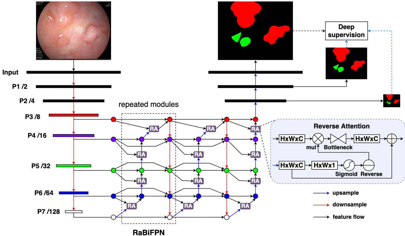
Figure 1: The overall architecture of our RaBiT contains two components: a lightweight MiT based encoder and a RaBiFPN decoder.
图 1: 我们的RaBiT整体架构包含两个组件:基于轻量级MiT的编码器和RaBiFPN解码器。
Inspired by these approaches for modeling multi-scale and multi-level features, we propose a new Transformer-based network called RaBiT. Our approach differs from the available models in several ways. In brief, our main contributions are fourfold. 1) In RaBiT, we design the encoder as a hierarchically structured lightweight Transformer for learning multi-scale features, and the decoder as a stack of bidirectional feature pyramid modules for learning from heterogeneous data containing feature maps extracted from encoder blocks at different scales and subregions; 2) A lightweight binary RA module using bottleneck layers is proposed to allow the repetition of this module several times in the stack of bidirectional feature pyramid layers to refine the segmentation boundaries of polyps increment ally; 3) A multi-class RA module is introduced, that is naturally suitable for multi-class segmentation; 4) An extensive set of experiments has been conducted on several standard benchmark datasets for polyp segmentation, and the results are compared with state-of-the-art methods.
受这些多尺度多层次特征建模方法的启发,我们提出了一种名为RaBiT的新型基于Transformer的网络。我们的方法在以下几个方面区别于现有模型:
- 在RaBiT中,我们将编码器设计为分层结构的轻量级Transformer用于学习多尺度特征,解码器则采用堆叠式双向特征金字塔模块,用于从包含不同尺度和子区域编码器块提取的特征图的异构数据中学习;
- 提出了一种使用瓶颈层的轻量级二元RA模块,该模块可在双向特征金字塔层堆叠中多次重复,以逐步细化息肉分割边界;
- 引入了天然适用于多类分割任务的多类RA模块;
- 在多个息肉分割标准基准数据集上进行了大量实验,并与最先进方法进行了结果对比。
The rest of the paper is organized as follows. First, the RaBiT architecture is described in Section 2. Next, Section 3 presents our experiments and results. Finally, we conclude the paper and highlight future works in Section 4.
本文的其余部分组织如下。首先,第2节介绍了RaBiT架构。接着,第3节展示了我们的实验和结果。最后,我们在第4节对全文进行总结并展望未来工作。
2 Method
2 方法
Our proposed network consists of a Transformer-based encoder and a decoder with a bidirectional feature pyramid network using consecutive RA modules. Therefore, we call our network RaBiT. The overall architecture of RaBiT is depicted in Fig. 1. Details will be given in the following sections.
我们提出的网络由一个基于Transformer的编码器和一个带有双向特征金字塔网络的解码器组成,该解码器使用了连续的RA模块。因此,我们将该网络命名为RaBiT。RaBiT的整体架构如图1所示,具体细节将在后续章节中介绍。
2.1 Encoder
2.1 编码器
Mix Transformer (MiT) [20] provides a hierarchical feature representation solution, which was designed to generate CNN-like multi-scale features. MiT has a series of variants, from MiT-B1 to MiT-B5, with the same architecture but different sizes. For efficiency, MiT-B3 is used as the backbone of our network for all experiments in this paper. Let $P_{i}$ be the feature map with a resolution of $1/2^{i}$ of the input images. The MiT encoder has five feature levels $P_{1}-P_{5}$ . Inspired by [9], to capture more multi-scale features, we derive two new feature levels $P_{6}$ and $P_{7}$ from $P_{5}$ . In order to obtain $P_{6}$ , we pass the feature map $P_{5}$ through a 1x1 conv layer with 224 neurons and stride 1, followed by a batch norm and a 3x3 max pooling layer with stride 2. Next, a 3x3 max pooling layer is applied to the feature map $P_{6}$ to get the feature map $P_{7}$ . Finally, all feature maps $P_{3}-P_{7}$ are fed to the decoder of the networks.
Mix Transformer (MiT) [20] 提供了一种分层特征表示方案,旨在生成类似CNN的多尺度特征。MiT有一系列变体,从MiT-B1到MiT-B5,架构相同但规模不同。出于效率考虑,本文所有实验均采用MiT-B3作为网络主干。设 $P_{i}$ 为输入图像分辨率 $1/2^{i}$ 的特征图。MiT编码器包含五个特征层级 $P_{1}-P_{5}$ 。受[9]启发,为捕获更多多尺度特征,我们从 $P_{5}$ 衍生出两个新特征层级 $P_{6}$ 和 $P_{7}$ 。为获得 $P_{6}$ ,我们将特征图 $P_{5}$ 通过具有224个神经元、步长1的1x1卷积层,随后接批量归一化和步长2的3x3最大池化层。接着对特征图 $P_{6}$ 应用3x3最大池化层得到 $P_{7}$ 。最终,所有特征图 $P_{3}-P_{7}$ 都被输入网络解码器。
2.2 Decoder
2.2 解码器
The decoder of RaBiT is designed to leverage the strengths of both BiFPN [9] and RA module [14]. The original RA [14] is employed in bottom-up direction to refine polyp boundaries, starting from the coarsest feature maps and progressing toward finer low-level ones. Inspired by BiFPN [9], we propose to iterative ly refine the polyp boundaries using RA. After each round of bottom-up refinement, we continue to fuse information between feature levels in a top-down direction. We then repeat the bottom-up polyp boundary refinement process and continue this procedure several times. We refer to the combination of top-down feature aggregation and bottom-up boundary refinement as a Reverse Attention based Bidirectional Feature Pyramid Network (RaBiFPN) module, which can be iterated multiple times to form a stacked block. In this paper, we repeat the RaBiFPN module four times based on our ablation studies. All feature maps in the decoder are aggregated using fast normalized fusion [9], where fusion weights are learned by back-propagation during the training phase. Eventually, we incorporate a last refinement branch to produce the final prediction (see Fig. 1).
RaBiT的解码器设计旨在结合BiFPN [9]和RA模块 [14]的优势。原始RA [14]采用自底向上的方向细化息肉边界,从最粗糙的特征图开始,逐步向更精细的低层特征图推进。受BiFPN [9]启发,我们提出使用RA迭代优化息肉边界。在每轮自底向上细化后,继续以自顶向下的方式融合各层级特征信息。随后重复自底向上的息肉边界细化过程,并多次迭代该流程。我们将这种自顶向下特征聚合与自底向上边界细化的组合称为基于反向注意力的双向特征金字塔网络 (RaBiFPN) 模块,该模块可多次迭代形成堆叠结构。根据消融实验,本文重复四次RaBiFPN模块。解码器中所有特征图均采用快速归一化融合 [9]进行聚合,其融合权重通过训练阶段的反向传播学习获得。最终通过最后一级细化分支生成预测结果 (见图1)。
The original RA module [14] takes an input and produces an output of size $H\times W\times1$ , and all the polyp boundary refinement steps are performed on single-channel feature maps. Compressing all feature maps into a single channel may result in the loss of critical information, reducing the effectiveness of multi-level feature fusion. In addition, single-channel processing is unsuitable for multi-class segmentation tasks, as each class must be processed separately in different channels. To address these limitations, we introduce a modified RA module that operates on feature maps of size $H\times W\times C$ , where $C=224$ is the number of channels in the last feature map $(P_{7})$ . Before being fed into the decoder, we use a 3x3 conv layer with $C$ neurons to compress the higher resolution feature maps from $P_{3}$ to $P_{5}$ to the same depth of $C=224$ . In contrast, the feature maps $P_{6}$ and $P_{7}$ have $C$ channels and can be fed directly to the decoder.
原始RA模块[14]接收输入并生成尺寸为$H\times W\times1$的输出,所有息肉边界细化步骤均在单通道特征图上执行。将全部特征图压缩至单通道可能导致关键信息丢失,降低多级特征融合效果。此外,单通道处理不适用于多类别分割任务,因为每个类别需要在不同通道中单独处理。为解决这些限制,我们改进的RA模块可处理尺寸为$H\times W\times C$的特征图,其中$C=224$对应末层特征图$(P_{7})$的通道数。在输入解码器前,我们使用含$C$个神经元的3x3卷积层,将$P_{3}$至$P_{5}$的高分辨率特征图压缩至相同深度$C=224$。而$P_{6}$和$P_{7}$特征图本身具有$C$个通道,可直接输入解码器。
For binary segmentation, we use a $3\mathrm{x}3$ conv layer with one neuron to compress the input feature map to a single channel. We then apply a sigmoid function followed by a reverse operation to perform RA for a single polyp class (see Fig. 1). For multi-class segmentation, we use a 3x3 conv layer with $n$ neurons to compress the input feature map to $n$ channels, where $n$ is the number of classes. We then apply a softmax function to generate an attention map for each channel. Next, each attention map is reversed to produce a reverse attention map and element-wise multiplied with the input feature map. Finally, the resulting feature maps are concatenated to form a $H\times W\times n C$ volume (see Fig. 2). To avoid parameter explosion when repeating the RA module multiple times in the network, we propose using a bottleneck module when performing the convolution operation to obtain the output feature map of the RA module. The bottleneck module consists of a 1x1 conv layer with $C/2$ neurons, followed by a 3x3 conv layer with $C/2$ neurons, and ends with a 1x1 conv layer with $C$ neurons.
对于二值分割任务,我们采用一个包含单神经元的$3\mathrm{x}3$卷积层将输入特征图压缩为单通道,随后通过Sigmoid函数及反向操作对单一息肉类别执行反向注意力机制(RA)(见图1)。在多类别分割场景中,我们使用含$n$个神经元的3x3卷积层将输入特征图压缩至$n$个通道(其中$n$为类别数),通过Softmax函数生成各通道的注意力图。每个注意力图经反向处理后与输入特征图进行逐元素相乘,最终将所得特征图拼接形成$H\times W\times n C$维度的特征体(见图2)。为避免在网络中多次重复RA模块导致的参数量爆炸,我们提出在卷积运算时采用瓶颈模块来获取RA模块的输出特征图。该瓶颈模块由含$C/2$个神经元的1x1卷积层、含$C/2$个神经元的3x3卷积层以及含$C$个神经元的1x1卷积层依次构成。
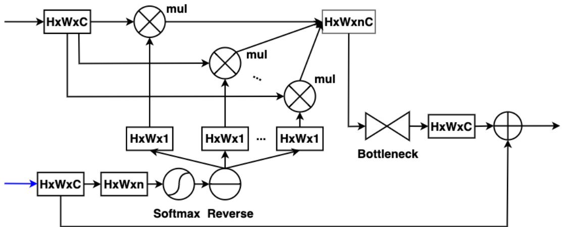
Figure 2: The architecture of Softmax RA module for multi-class segmentation.
图 2: 用于多类分割的Softmax RA模块架构。
2.3 Loss Function
2.3 损失函数
For binary segmentation, we use a compound loss combining a weighted focal loss and a weighted IoU loss. Similar to PraNet [14], the weighted losses are used to increase the weights of hard pixels. However, unlike PraNet, we utilize the focal loss [21] instead of BCE to deal with the imbalanced data problem in polyp segmentation. For multi-class polyp segmentation, the categorical cross-entropy loss is used. Finally, we also apply deep supervision to multi-scale outputs to train the network, as shown in Fig. 1. The final loss is the sum of all losses computed at the different output levels. Note that each output is upsampled back to the original size of the image’s ground truth before the losses are calculated.
对于二分类任务,我们采用加权焦点损失 (focal loss) 与加权交并比损失 (IoU loss) 的复合损失函数。与PraNet [14] 类似,加权损失用于增强困难像素的权重。但不同于PraNet,我们使用焦点损失 [21] 替代二元交叉熵 (BCE) 来解决息肉分割中的类别不平衡问题。在多分类息肉分割任务中,则采用分类交叉熵损失。如图 1 所示,我们还在多尺度输出上应用深度监督机制来训练网络。最终损失函数为各层级输出损失的求和结果。需注意,在计算损失前,每个输出都会上采样至原始标注图像的尺寸。
3 Experiments
3 实验
3.1 Datasets
3.1 数据集
We conducted experiments on five popular datasets for binary polyp segmentation: Kvasir [22], CVC-Clinic DB [23], CVC-Colon DB [24], CVC-T [25], and ETIS-Larib Polyp DB [26]. We then compared our approach with existing methods on two datasets for multi-class polyp segmentation, NeoPolyp-Large and NeoPolyp-Small [13], where the challenging goal is not only to segment polyps from the background but also to determine benign and neoplastic polyps.
我们在五个流行的二进制息肉分割数据集上进行了实验:Kvasir [22]、CVC-Clinic DB [23]、CVC-Colon DB [24]、CVC-T [25] 和 ETIS-Larib Polyp DB [26]。随后,我们在两个多类别息肉分割数据集(NeoPolyp-Large 和 NeoPolyp-Small [13])上将我们的方法与现有方法进行了比较,这两个数据集的挑战性目标不仅是从背景中分割息肉,还要区分良性和肿瘤性息肉。
Table 1: Performance comparison for binary polyp segmentation.
表 1: 二分类息肉分割性能对比
| 方法 | Kvasir | CVC-ClinicDB | CVC-ColonDB | CVC-T | ETIS-Larib | |||||
|---|---|---|---|---|---|---|---|---|---|---|
| mDice | mIoU | mDice | mIoU | mDice | mIoU | mDice | mIoU | mDice | mIoU | |
| UNet [6] | 0.818 | 0.746 | 0.823 | 0.750 | 0.512 | 0.444 | 0.710 | 0.627 | 0.398 | 0.335 |
| UNet++ [11] | 0.821 | 0.743 | 0.794 | 0.729 | 0.483 | 0.410 | 0.707 | 0.624 | 0.401 | 0.344 |
| SFA [27] | 0.723 | 0.611 | 0.700 | 0.607 | 0.469 | 0.347 | 0.297 | 0.217 | 0.467 | 0.329 |
| PraNet [14] | 0.898 | 0.840 | 0.899 | 0.849 | 0.709 | 0.640 | 0.871 | 0.797 | 0.628 | 0.567 |
| HarDNet-MSEG[7] | 0.912 | 0.857 | 0.932 | 0.882 | 0.731 | 0.660 | 0.887 | 0.821 | 0.677 | 0.613 |
| TransUNet [18] | 0.913 | 0.857 | 0.935 | 0.887 | 0.781 | 0.699 | 0.893 | 0.824 | 0.731 | 0.660 |
| CaraNet [15] | 0.918 | 0.865 | 0.936 | 0.887 | 0.773 | 0.689 | 0.903 | 0.838 | 0.747 | 0.672 |
| TransFuse-L*[19] | 0.920 | 0.870 | 0.942 | 0.897 | 0.781 | 0.706 | 0.894 | 0.826 | 0.737 | 0.663 |
| RaBiT (Ours) | 0.927 | 0.879 | 0.936 | 0.890 | 0.824 | 0.749 | 0.905 | 0.839 | 0.823 | 0.747 |
Table 2: Performance comparison for multi-class polyp segmentation.
表 2: 多类别息肉分割性能对比
| Method | NeoPolyp-Large | NeoPolyp-Small | |||||
|---|---|---|---|---|---|---|---|
| Diceseg | IoUseg | Dicenon | IoUnon | Diceneo | IoUneo | Kaggle score | |
| UNet [6] | 0.785 | 0.646 | 0.525 | 0.356 | 0.773 | 0.631 | |
| ColonSegNet [4] | 0.738 | 0.585 | 0.505 | 0.338 | 0.732 | 0.577 | |
| DDANet [5] | 0.813 | 0.684 | 0.578 | 0.406 | 0.802 | 0.670 | |
| DoubleU-Net [12] | 0.837 | 0.720 | 0.621 | 0.450 | 0.832 | 0.712 | |
| HarDNet-MSEG [7] | 0.883 | 0.791 | 0.659 | 0.492 | 0.869 | 0.769 | |
| PraNet [14] | 0.895 | 0.811 | 0.705 | 0.544 | 0.873 | 0.775 | |
| BlazeNeo-DHA [8] | 0.904 | 0.825 | 0.717 | 0.559 | 0.885 | 0.792 | 0.788 |
| NeoUNet [13] | 0.911 | 0.837 | 0.720 | 0.563 | 0.889 | 0.800 | 0.807 |
| RaBiT (Ours) | 0.940 | 0.886 | 0.765 | 0.619 | 0.917 | 0.846 | 0.859 |
3.2 Experiment Settings and Metrics
3.2 实验设置与评估指标
We implemented RaBiT using PyTorch. We trained the networks on a machine with 64GB RAM and an RTX 3090 GPU. Input images were resized to $384\times384$ . We employed a multi-scale training strategy with scales of ${256,384$ , $512}$ . Standard augmentation techniques were used, such as horizontal/vertical flip, random rotation of $90^{\circ}$ , gaussian blur, color jitter, and random crop. We used the Adam optimizer and cosine annealing scheduler with a learning rate of 1e-4. RaBiT was trained in 30 epochs with a batch size of 8, and the last checkpoint was used for evaluation. We trained RaBiT five times, and results (except for the last column in Table 2) were averaged over five runs for all experiments.
我们使用PyTorch语言实现了RaBiT。训练在一台配备64GB内存和RTX 3090 GPU的机器上进行。输入图像尺寸调整为$384\times384$。采用了多尺度训练策略,尺度为${256,384$, $512}$。使用了标准数据增强技术,包括水平/垂直翻转、$90^{\circ}$随机旋转、高斯模糊、色彩抖动和随机裁剪。优化器选用Adam,学习率设为1e-4,并采用余弦退火调度器。RaBiT训练30个epoch,批量大小为8,最终评估使用最后一个检查点。所有实验均进行五次训练,结果(表2最后一列除外)取五次运行的平均值。
We set up two groups of experiments to evaluate our method. 1) Binary polyp segmentation: We used the same split as suggested in [14], where $90%$ of the Kvasir and ClinicDB datasets were used for training. The remaining images in the Kvasir and CVC-ClinicDB datasets were used for testing, and all from CVC-ColonDB, CVC-T, and ETIS-Larib were used for cross-dataset testing; 2) Multi-class polyp segmentation: we used the NeoPolyp-Large dataset and followed the data split in [13]. We also used a reduced version called NeoPolyp-Small [28] for comparing different methods.
我们设置了两组实验来评估我们的方法。1) 二分类息肉分割:采用与[14]相同的划分方式,使用Kvasir和ClinicDB数据集中90%的数据进行训练。Kvasir和CVC-ClinicDB数据集中剩余的图像用于测试,而CVC-ColonDB、CVC-T和ETIS-Larib的全部数据用于跨数据集测试;2) 多类别息肉分割:使用NeoPolyp-Large数据集并遵循[13]的数据划分。我们还使用了一个精简版本NeoPolyp-Small [28]来比较不同方法。
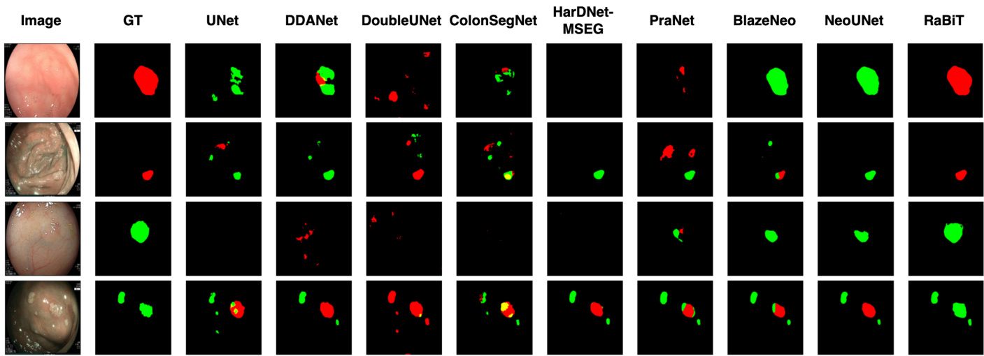
Figure 3: Qualitative result comparison on the Neo-Large dataset.
图 3: Neo-Large数据集上的定性结果对比。
Similar to [14], we employ the mDice and mIoU metrics for quantitative evaluation of binary polyp segmentation. For multi-class polyp segmentation, we calculate micro mDice and micro mIoU for neoplastic, non-neoplastic, and generic polyps, respectively, as suggested in [13]. Besides, since the test set of the Neo Neo Polyp-Small dataset is not public, we use the Kaggle mDice score described in [28] to compare different methods on the Kaggle leader board.
与[14]类似,我们采用mDice和mIoU指标对息肉二分类分割进行定量评估。对于多类别息肉分割,按照[13]的建议,我们分别计算肿瘤性、非肿瘤性和通用息肉类别的微观mDice和微观mIoU值。此外,由于Neo Polyp-Small数据集的测试集未公开,我们采用[28]所述的Kaggle mDice分数来比较Kaggle排行榜上的不同方法。
3.3 Comparison with the State-of-the-art (SOTA) Methods
3.3 与最先进 (SOTA) 方法的对比
The performance comparison for binary polyp segmentation is described in Table 1. RaBiT generally outperforms the benchmark models on most datasets. RaBiT outperforms the second-best TransFuse $\mathbf{-L}^{}$ by $4.3%$ in mDice and $4.3%$ in mIoU on CVC-ColonDB. Notably, RaBiT achieves a significant improvement of $7.6%$ in mDice and $7.5%$ in mIoU compared to the second-best CaraNet [15] on ETIS-Larib. The efficacy of the RaBiFPN module within RaBiT appears to be well-suited for the high-resolution images in ETIS-Larib. However, RaBiT has roughly $0.7%$ lower metric values than the best TransFuse $\mathbf{-L}^{*}$ on CVC-ClinicDB, which contains low-resolution images.
表1描述了二进制息肉分割的性能对比。RaBiT在大多数数据集上普遍优于基准模型。在CVC-ColonDB上,RaBiT以mDice提升4.3%、mIoU提升4.3%的表现超越次优的TransFuse $\mathbf{-L}^{}$。值得注意的是,在ETIS-Larib数据集上,RaBiT相比次优的CaraNet [15]实现了mDice 7.6%和mIoU 7.5%的显著提升。RaBiT中的RaBiFPN模块似乎特别适合处理ETIS-Larib中的高分辨率图像。然而,在包含低分辨率图像的CVC-ClinicDB上,RaBiT的指标值比最优的TransFuse $\mathbf{-L}^{*}$低约0.7%。
Table 2 shows the performance comparison of SOTA methods on three-class polyp segmentation datasets. RaBiT outperforms the second-best method, NeoUNet [13], for every metric by a large margin of about $3%.6%$ . Fig. 7 shows the qualitative comparison between our approach and other SOTA methods on the NeoPolyp-Large dataset. One can see that RaBiT yields better segmentation results than other SOTA methods in many challenging cases.
表 2 展示了三类息肉分割数据集上 SOTA (state-of-the-art) 方法的性能对比。RaBiT 以约 $3%\sim6%$ 的显著优势在所有指标上均优于第二名 NeoUNet [13]。图 7 展示了我们的方法与其他 SOTA 方法在 NeoPolyp-Large 数据集上的定性对比结果。可以看出,在许多具有挑战性的案例中,RaBiT 能产生比其他 SOTA 方法更优的分割结果。
3.4 Learning Capability
3.4 学习能力
To better evaluate the learning capability of our method, we conducted 5-fold cross-validation on the CVC-ClinicDB and Kvasir datasets. Each dataset is divided into five equal folds. Each run uses one fold for testing and four remaining folds for training. Table 3 describes the comparison results for this experiment. The average value and standard deviation are used as metrics to prove the models’ stability. Our RaBiT not only outperforms all other state-of-the-art models in mDice, mIoU, precision, and recall on both datasets but also is the most stable model on both datasets, achieving the lowest standard deviation for each evaluation metric.
为了更好评估我们方法的学习能力,我们在CVC-ClinicDB和Kvasir数据集上进行了5折交叉验证。每个数据集被均分为五份。每次实验使用其中一份作为测试集,其余四份作为训练集。表3描述了本实验的对比结果。采用平均值和标准差作为衡量模型稳定性的指标。我们的RaBiT不仅在两个数据集的mDice、mIoU、精确率和召回率上均优于其他最先进模型,同时是这两个数据集上最稳定的模型,各项评估指标的标准差均为最低。
Qualitative results for this experiment are shown in Fig. 4. RaBiT demonstrates much fewer wrongly predicted pixel in segmentation results than other models.
该实验的定性结果如图4所示。RaBiT在分割结果中展示的错误预测像素远少于其他模型。
Table 3: Performance comparison of different methods on 5-fold cross-validation of the CVC-ClinicDB and Kvasir datasets. All results are averaged over five folds.
表 3: CVC-ClinicDB和Kvasir数据集五折交叉验证中不同方法的性能对比。所有结果为五折平均值。
| 数据集 | 方法 | mDice | mIoU | Recall | Precision |
|---|---|---|---|---|---|
| CVC-ClinicDB | UNet [6] | 0.792 | |||
| MultiResUNet [29] | 0.849 | ||||
| ResUNet++ [30] | 0.815 ± 0.018 | 0.736 ± 0.017 | 0.832 ± 0.018 | 0.830 ± 0.020 | |
| DoubleUNet [12] | 0.920 ± 0.018 | 0.866 ± 0.025 | 0.922 ± 0.027 | 0.928 ± 0.017 | |
| DDANet [5] ColonSegNet [4] HarDNet-MSEG [7] | 0.860 ± 0.014 0.817 ± 0.020 | 0.786 ± 0.017 0.873 ± 0.024 | 0.858 ± 0.023 0.926 ± 0.025 | 0.892 ± 0.014 0.933 ± 0.014 | |
| PraNet [14] RaBiT (Ours) UNet [6] ResUNet++ [30] | 0.923 ± 0.020 0.933 ± 0.012 | 0.873 ± 0.024 0.884 ± 0.015 | 0.926 ± 0.025 0.940 ± 0.005 | 0.933 ± 0.014 0.937 ± 0.016 | |
| 0.911 ± 0.002 | 0.949 ± 0.003 | 0.956 ± 0.002 | |||
| 0.951 ± 0.002 | |||||
| 0.708 ± 0.017 | 0.602 ± 0.010 | 0.805 ± 0.014 | 0.716 ± 0.020 | ||
| 0.780 ± 0.010 | 0.681 ± 0.008 | 0.834 ± 0.010 | 0.799 ± 0.010 | ||
| Kvasir | RaBiT (Ours) DoubleUNet [12] HarDNet-MSEG [7] PraNet [14] | ||||
| DDANet [5] | 0.879 ± 0.018 0.860 ± 0.005 | 0.816 ± 0.026 | 0.902 ± 0.027 | 0.894 ± 0.039 | |
| ColonSegNet [4] | 0.791 ± 0.004 | 0.876 ± 0.015 | 0.892 ± 0.018 | ||
| 0.676 ± 0.037 | 0.557 ± 0.040 | 0.731 ± 0.088 | 0.730 ± 0.080 | ||
| 0.889 ± 0.011 0.883 ± 0.020 | 0.831 ± 0.011 | 0.822 ± 0.020 0.897 ± 0.020 | 0.892 ± 0.015 |
3.5 Generalization Capability
3.5 泛化能力
To better evaluate the generalization capability, we conducted additional experiments with the following configurations:
为了更全面地评估泛化能力,我们进行了以下配置的补充实验:
Table 4 shows the comparison results for these experiments. Overall, RaBiT significantly outperforms benchmark models on every cross-dataset metric. For the first configuration, RaBiT outperforms the second-best PraNet by $6.8%$ on mDice and $8.3%$ on mIoU. In the second configuration, RaBiT continues to achieve a $9.7%$ improvement in recall, $5.8%$ improvement in mDice, and $6.8%$ improvement in mIoU over PraNet. Especially for the third configuration, RaBiT again shows its suitability to the ETIS-Larib dataset achieving a $15%$ improvement in mDice, $14.5%$ in mIoU, $10%$ in recall and $19.5%$ in precision over the second-best HarDNet-MSEG. These are highly significant improvements, showing that our RaBiT can generalize well to new unseen data. Some result samples for this experiment are shown in Fig. 5. Similar to Fig. 4, one can see that RaBiT produces better segmentation results than other state-of-the-art.
表 4 展示了这些实验的对比结果。总体而言,RaBiT 在每项跨数据集指标上都显著优于基准模型。在第一种配置下,RaBiT 在 mDice 上比第二名的 PraNet 高出 $6.8%$ ,在 mIoU 上高出 $8.3%$ 。第二种配置中,RaBiT 继续实现比 PraNet 高 $9.7%$ 的召回率提升、 $5.8%$ 的 mDice 提升以及 $6.8%$ 的 mIoU 提升。特别是在第三种配置下,RaBiT 再次展现出对 ETIS-Larib 数据集的适配性,在 mDice 上比第二名的 HarDNet-MSEG 高出 $15%$ ,mIoU 高出 $14.5%$ ,召回率高出 $10%$ ,精确度高出 $19.5%$ 。这些改进具有高度显著性,表明我们的 RaBiT 能够很好地泛化到未见过的数据。该实验的部分结果样本如图 5 所示。与图 4 类似,可以看出 RaBiT 比其他最先进方法产生了更好的分割结果。

Figure 4: Qualitative result comparison of different models trained on the first fold of the 5-fold cross-validation on the Kvasir dataset.
图 4: 在Kvasir数据集上使用5折交叉验证第一折训练的不同模型的定性结果对比。

Figure 5: Qualitative result comparison using CVC-Colon for training and CVC-Clinic for testing.
图 5: 使用CVC-Colon训练和CVC-Clinic测试的定性结果对比。
Table 4: Performance comparison of different methods on cross-dataset configurations. All results are averaged over five runs.
表 4: 跨数据集配置下不同方法的性能对比。所有结果为五次运行的平均值。
| 训练集 | 测试集 | 方法 | mDice | mIoU | Recall | Precision |
|---|---|---|---|---|---|---|
| VC-ColonDB ETIS-Larib + | -ClinicDB | ResUNet++ [30] ColonSegNet [4] DDANet [5] DoubleUNet [12] HarDNet-MSEG [7] PraNet [14] RaBiT (Ours) | 0.406 0.427 0.624 0.738 0.765 0.779 0.847 | 0.302 0.321 0.515 0.651 0.681 0.689 0.772 | 0.481 0.529 0.697 0.758 0.774 0.832 0.894 | 0.496 0.552 0.692 0.824 0.863 0.812 |
| -ColonDB | ClinicDB | ResUNet++ [30] DoubleUNet [12] DDANet [5] ResNet101-Mask-RCNN [31] ColonSegNet [4] HarDNet-MSEG [7] PraNet [14] RaBiT (Ours) | 0.339 0.441 0.476 0.641 0.582 0.721 0.738 0.796 0.211 | 0.247 0.375 0.370 0.565 0.268 0.633 0.647 0.715 | 0.380 0.423 0.501 0.646 0.511 0.744 0.751 0.848 | 0.857 0.484 0.639 0.644 0.725 0.460 0.818 0.832 0.820 |
| -ClinicDB 2 | ETIS-Larib | ResUNet++ [30] ColonSegNet [4] DDANet [5] ResNet101-Mask-RCNN [31] DoubleUNet [12] PraNet [14] HarDNet-MSEG [7] RaBiT (Ours) | 0.217 0.400 0.565 0.588 0.631 0.659 0.809 | 0.155 0.110 0.313 0.469 0.500 0.555 0.583 0.728 | 0.309 0.654 0.507 0.565 0.689 0.762 0.676 0.776 | 0.203 0.144 0.464 0.639 0.599 0.597 0.705 0.900 |
3.6 Adaptation Capability to other Medical Image Segmentation Tasks
3.6 对其他医学图像分割任务的适应能力
We demonstrate the generalization capability of our method to other medical image analysis tasks by conducting an experiment on the ISIC 2018 dataset for skin lesion segmentation. Results are shown in Table 5. One can see that our RaBiT yields superior performance compared to other state-of-the-art methods. This suggests that our RaBiT can serve as a strong baseline for other medical image segmentation tasks.
我们通过在ISIC 2018皮肤病变分割数据集上进行实验,验证了该方法对其他医学图像分析任务的泛化能力。结果如表5所示。可以看出,我们的RaBiT相比其他最先进方法具有更优性能,这表明RaBiT能够作为其他医学图像分割任务的强基准。
Table 5: Performance comparison of different methods on ISIC-2018 dataset.
表 5: ISIC-2018数据集上不同方法的性能对比。
| 方法 | mDice | Precision | Recall | Accuracy |
|---|---|---|---|---|
| UNet [6] | 0.647 | 0.779 | 0.708 | 0.890 |
| AttentionUNet [10] | 0.665 | 0.787 | 0.717 | 0.897 |
| R2U-Net [32] | 0.679 | 0.741 | 0.792 | 0.880 |
| AttentionR2U-Net | 0.691 | 0.822 | 0.726 | 0.904 |
| BCDU-Net(d=3) [33] | 0.851 | 0.928 | 0.785 | 0.937 |
| MCGU-Net(d=3) [34] | 0.895 | 0.947 | 0.848 | 0.955 |
| RaBiT (Ours) | 0.904 | 0.917 | 0.916 | 0.964 |
3.7 Complexity Comparison
3.7 复杂度对比
Table 6 compares RaBiT with other benchmark models in terms of size and computational complexity. Our RaBiT obtains competitive size and computational complexity compared to the most lightweight CNN-based models such as
表 6: 对比RaBiT与其他基准模型的参数量及计算复杂度。我们的RaBiT与最轻量级的CNN模型相比,在参数量和计算复杂度方面均具有竞争力,例如
PraNet [14], and HarDNet-MSEG [7]. RaBiT is larger than most CNN-based neural networks but still more efficient than other Transformer-based methods in terms of GFlops.
PraNet [14] 和 HarDNet-MSEG [7]。RaBiT 比大多数基于 CNN 的神经网络更大,但在 GFlops 方面仍比其他基于 Transformer 的方法更高效。
Fig. 6 shows that the bottleneck module reduces the number of parameters and GFlops by about half compared to the same RaBiT network without using it. The bottleneck module also allows the repetition of RaBiFPN blocks without a negligible increase in the number of parameters and GFlops of the network.
图 6 显示,与未使用瓶颈模块的相同 RaBiT 网络相比,该模块将参数量和 GFlops 减少了约一半。瓶颈模块还允许重复 RaBiFPN 块,而不会导致网络参数量和 GFlops 出现显著增加。
Table 6: Number of parameters and GFLOPs of different methods
表 6: 不同方法的参数量和GFLOPs对比
| 方法 | 参数量 (M) | GFLOPs |
|---|---|---|
| PraNet [14] | 32.55 | 13.11 |
| HarDNet-MSEG [7] | 33.34 | 11.38 |
| CaraNet [15] | 46.64 | 21.69 |
| TransUNet [18] | 105.5 | 60.75 |
| TransFuse-L* [19] | ||
| SegFormer-B3 [20] | 47.22 | 33.68 |
| RaBiTw/bottleneck | 51.72 | 23.12 |
| RaBiTw/obottleneck | 81.79 | 41.37 |
3.8 Ablation Studies
3.8 消融实验
Effectiveness of the RaBiFPN and the bottleneck modules. We evaluated the effectiveness of these modules through the generalization capability of the models on unseen data. We followed the setup for the first experimental group in Section 3.2 to compare RaBiT with SegFormer-B3 [20], which employs the original weighted BiFPN module [9]. Both models leverage the same MiT-B3 backbone as the encoder.
RaBiFPN和瓶颈模块的有效性。我们通过模型在未见数据上的泛化能力评估了这些模块的有效性。按照第3.2节第一实验组的设置,将采用原始加权BiFPN模块[9]的SegFormer-B3 [20]与RaBiT进行对比。两个模型均使用相同的MiT-B3骨干网络作为编码器。
Table 7: Ablation study on the effectiveness of the RaBiFPN and bottleneck modules on the unseen data.
表 7: 在未见数据上对RaBiFPN和瓶颈模块有效性的消融研究。
| wBiFPN | RaBiFPN | Bottleneck | CVC-ColonDB | CVC-ColonDB | CVC-T | CVC-T | ETIS-Larib | ETIS-Larib |
|---|---|---|---|---|---|---|---|---|
| mDice | mloU | mDice | mIoU | mDice | mloU | |||
| √ | 0.812 | 0.733 | 0.900 | 0.829 | 0.784 | 0.708 | ||
| √ | 0.820 | 0.746 | 0.905 | 0.840 | 0.828 | 0.753 | ||
| √ | √ | 0.824 | 0.749 | 0.905 | 0.839 | 0.823 | 0.747 |
Table 8: Evaluation metrics for different types of the RA module.
表 8: RA模块不同变体的评估指标
| 数据集 | 激活函数 | Diceseg | IoUseg | Dicenon | IoUnon | Diceneo | IoUneo |
|---|---|---|---|---|---|---|---|
| NeoPolyp-Large | sigmoid | 93.66 | 88.08 | 75.18 | 60.23 | 91.34 | 84.07 |
| softmax | 94.00 | 88.59 | 76.47 | 61.90 | 91.65 | 84.59 | |
| NeoPolyp-Small | sigmoid | 93.40 | 87.61 | 70.22 | 54.10 | 92.39 | 85.85 |
| softmax | 94.01 | 88.69 | 76.65 | 62.15 | 93.80 | 88.33 |
Table 7 shows the superior performance of the RaBiFPN module compared to the original BiFPN module. The mIoU improvement on the CVC-ColonDB and CVC-T datasets, which contain low-resolution images, is above $1%$ . However, the improvement on ETIS-Larib, containing high-resolution images, is up to $4.5%$ in mIoU. This observation emphasizes the increasing effectiveness of RaBiFPN as image size grows. Although the bottleneck module negligibly impacts performance for large images in ETIS-Larib, it slightly improves the performance on smaller images in CVCColonDB. Moreover, the bottleneck module also reduces our network’s parameters from 81.79M to 51.72M and decreases computational complexity from 41.37 GFlops to 23.12 GFlops.
表 7 展示了 RaBiFPN 模块相比原始 BiFPN 模块的卓越性能。在包含低分辨率图像的 CVC-ColonDB 和 CVC-T 数据集上,mIoU 提升超过 $1%$。而在包含高分辨率图像的 ETIS-Larib 数据集上,mIoU 提升高达 $4.5%$。这一观察结果强调了 RaBiFPN 随着图像尺寸增大而增强的有效性。尽管瓶颈模块对 ETIS-Larib 中的大尺寸图像性能影响可忽略不计,但它略微提升了 CVCColonDB 中小尺寸图像的性能。此外,瓶颈模块还将网络参数量从 81.79M 减少至 51.72M,并将计算复杂度从 41.37 GFlops 降低至 23.12 GFlops。
Effectiveness of the softmax RA module. We evaluated the performance of RaBiT using the sigmoid and softmax RA modules on the Neo-Small and Neo-Large datasets. Results in Table 8 show a consistent improvement when using softmax in the RA module for the multi-class polyp segmentation task. Overall, RaBiT with softmax RA improves results according to all metrics on all datasets. Especially, the ${\mathrm{Dice}}_{n o n}$ metric improves by $6.43%$ on the Neo-Small dataset. This observation suggests the increasing effectiveness of the softmax RA when dealing with small objects such as non-neoplastic polyps.
softmax RA模块的有效性。我们在Neo-Small和Neo-Large数据集上评估了RaBiT使用sigmoid和softmax RA模块的性能。表8结果显示,在多类别息肉分割任务中使用softmax RA模块能带来一致的性能提升。总体而言,采用softmax RA的RaBiT在所有数据集的所有指标上均有改善,其中Neo-Small数据集的${\mathrm{Dice}}_{n o n}$指标提升了$6.43%$。这一现象表明,softmax RA在处理非肿瘤性息肉等小目标时具有更高的有效性。
3.9 Ablation Study on the Number of RaBiFPN Modules
3.9 RaBiFPN模块数量的消融研究
We evaluate the performance of RaBiT with 2 - 4 - 6 RaBiFPN modules. Results are shown in Table 9. Overall, RaBiT with 4 RaBiFPN modules achieved the best result on most datasets except for the ETIS-Larib that contains high-resolution images. We also use RaBiT with 4 RaBiFPN modules in all other experiments in this paper.
我们评估了包含2至4个RaBiFPN模块的RaBiT性能,结果如表9所示。总体而言,配置4个RaBiFPN模块的RaBiT在多数数据集上表现最优(除包含高分辨率图像的ETIS-Larib外)。本文其余实验均采用4个RaBiFPN模块的RaBiT配置。
Table 9: Evaluation metrics for different numbers of RaBiFPN modules. All results are averaged over five runs.
表 9: 不同数量RaBiFPN模块的评估指标。所有结果为五次运行的平均值。
| #RaBiFPN模块 | Kvasir-mDice | Kvasir-mIoU | ClinicDB-mDice | ClinicDB-mIoU | ColonDB-mDice | ColonDB-mIoU | CVC-T-mDice | CVC-T-mIoU | ETIS-Larib-mDice | ETIS-Larib-mIoU |
|---|---|---|---|---|---|---|---|---|---|---|
| 2 | 0.926 | 0.878 | 0.933 | 0.887 | 0.822 | 0.749 | 0.902 | 0.836 | 0.824 | 0.746 |
| 4 | 0.927 | 0.879 | 0.936 | 0.890 | 0.824 | 0.749 | 0.905 | 0.839 | 0.823 | 0.747 |
| 6 | 0.922 | 0.872 | 0.935 | 0.888 | 0.822 | 0.745 | 0.902 | 0.836 | 0.827 | 0.750 |

Figure 6: Effect of repeating RaBiFPN modules on the number of parameters and GFlops of RaBiT.
图 6: 重复RaBiFPN模块对RaBiT参数量和GFlops的影响
4 Conclusion
4 结论
This paper proposes RaBiT, a new Transformer-based network for automatic and accurate segmentation of colon polyps. RaBiT incorporates a hierarchically structured lightweight Transformer in the encoder and a stack of bidirectional feature pyramid modules in the decoder with repeated lightweight RA modules for iterative polyp boundary refinement. Our method outperforms existing methods across several benchmark datasets for polyp segmentation while maintaining low computational complexity. Furthermore, our method demonstrates high generalization capability in cross-dataset experiments.
本文提出RaBiT,一种基于Transformer的新型网络,用于自动精确分割结肠息肉。RaBiT在编码器中采用分层结构的轻量级Transformer,在解码器中堆叠双向特征金字塔模块,并通过重复的轻量级RA模块迭代优化息肉边界。我们的方法在多个息肉分割基准数据集上超越现有方法,同时保持较低计算复杂度。此外,跨数据集实验表明该方法具有高度泛化能力。
In future works, we will exploit alternative feature aggregation mechanisms to improve the representation of high-level semantic features.
在未来的工作中,我们将探索替代性特征聚合机制以提升高层语义特征的表征能力。
References
参考文献
5 Appendices
5 附录
5.1 Details of Datasets
5.1 数据集详情
5.1.1 Binary polyp segmentation.
5.1.1 二元息肉分割
We conducted experiments for binary polyp segmentation on the two following datasets:
我们在以下两个数据集上进行了二分类息肉分割实验:
Kvasir dataset [22] collected using endoscopic equipment at Vestre Viken Health Trust (VV), Norway. Images were carefully annotated and verified by experienced g astro entero logi sts from VV and the Cancer Registry of Norway. The dataset consists of 1000 images with different resolutions from $720\times576$ to $1920\times1072$ pixels.
Kvasir数据集 [22] 由挪威Vestre Viken Health Trust (VV)通过内窥镜设备采集。所有图像均由VV和挪威癌症登记处的资深胃肠病专家进行细致标注与验证。该数据集包含1000张分辨率从$720\times576$到$1920\times1072$像素不等的图像。
CVC-ClinicDB dataset [23] a database of frames extracted from colon os copy videos. The dataset consists of 612 images with a resolution of $384\times288$ pixels from 31 colon os copy sequences. The dataset was used in the training stages of the MICCAI 2015 Sub-Challenge on Automatic Polyp Detection Challenge in Colon os copy Videos.
CVC-ClinicDB数据集 [23] 是一个从结肠镜视频中提取帧的数据库。该数据集包含31段结肠镜视频序列中的612张图像,分辨率为$384\times288$像素。该数据集被用于MICCAI 2015结肠镜视频自动息肉检测子挑战赛的训练阶段。
CVC-ColonDB dataset [24] is provided by the Machine Vision Group (MVG). The dataset consists of 380 images with a resolution of $574\times500$ pixels from 15 short colon os copy videos.
CVC-ColonDB数据集[24]由机器视觉组(MVG)提供。该数据集包含来自15段结肠镜短视频的380张图像,分辨率为$574\times500$像素。
CVC-T dataset [25] is the test set of a more extensive dataset called Endoscene. CVC-T consists of 60 images obtained from 44 video sequences acquired from 36 patients.
CVC-T数据集 [25] 是名为Endoscene的更广泛数据集的测试集。CVC-T包含从36名患者采集的44段视频序列中获取的60张图像。
ETIS-Larib dataset [26] contains 196 high resolution $(1226\times996)$ ) colon os copy images.
ETIS-Larib数据集 [26] 包含196张高分辨率 $(1226\times996)$ 结肠镜图像。
5.1.2 Multi-class polyp segmentation.
5.1.2 多类别息肉分割
We conducted experiments for multi-class polyp segmentation on the two following datasets:
我们在以下两个数据集上进行了多类别息肉分割实验:
NeoPolyp-Small [28] is a public dataset in a Kaggle competition. The dataset contains 1200 images. The training set consists of 1000 images, and the test set consists of 200 images.
NeoPolyp-Small [28] 是 Kaggle 竞赛中的一个公开数据集。该数据集包含 1200 张图像,其中训练集有 1000 张图像,测试集有 200 张图像。
NeoPolyp-Large [13] is a bigger version of the NeoPolyp-Small. The training set has 5277 images, and the test set has 1353 images.
NeoPolyp-Large [13] 是 NeoPolyp-Small 的更大版本。训练集包含 5277 张图像,测试集包含 1353 张图像。
5.2 Qualitative Comparison for Multi-class Polyp Segmentation
5.2 多类别息肉分割的定性比较
Fig. 7 shows more examples of the qualitative comparison between our approach and other state-of-the-art methods on the NeoPolyp-Large dataset. One can see that RaBiT yields more precise segmentation results than other state-ofthe-art.
图7展示了我们的方法与其他先进方法在NeoPolyp-Large数据集上的更多定性对比示例。可以看出,RaBiT比其他先进方法产生了更精确的分割结果。

Figure 7: Qualitative result comparison in Neo-Large dataset.
图 7: Neo-Large数据集中的定性结果对比。
5.3 Details of Data Augmentation
5.3 数据增强细节
5.3.1 Binary polyp segmentation
5.3.1 二进制息肉分割
Each image has a probability of $50%$ to be augmented by the sequence of the following transforms:
每张图像有 50% 的概率通过以下变换序列进行增强:
The probability of applying each of these transforms is $50%$ , except for the crop transform, which has a probability of $20%$ . All augmented images are then resized back to the input size of $384\mathrm{x}384$ after the augmentation steps. Below are the codes for data augmentation using the albumen tat ions python library:
应用每种变换的概率为$50%$,裁剪变换除外,其概率为$20%$。所有增强后的图像在增强步骤完成后会调整回输入尺寸$384\mathrm{x}384$。以下是使用albumentations Python库进行数据增强的代码:
i m a g e t r a n s f o r m $=$ Compose ( [ r o t a t e . Random Rotate 90 ( ) ,
图像变换 (image transform) = 组合 ( [旋转.随机旋转90度 ( ) ,
t r a n s f o r m s . F l i p ( ) , t r a n s f o r m s . H u e S a t u r a t i o n V a l u e ( ) , t r a n s f o r m s . R a n d o m B r i g h t n e s s C o n t r a s t ( ) , t r a n s f o r m s . G a u s s i a n B l u r ( ) , t r a n s f o r m s . T r a n s p o s e ( ) , OneOf ( [ c r o p . RandomCrop ( 2 2 4 , 224 , $\mathsf{p}=\mathsf{l}$ ) , c r o p . C e n t e r C r o p ( 2 2 4 , 2 2 4 , $\mathsf{p}{=}1$ ) ] , $\mathfrak{p}{=}0.2)$ , r e s i z e . R e s i z e ( HEIGHT , HEIGHT ) ] , $\mathrm{p}{=}0.5\$ )
transforms.Flip(), transforms.HueSaturationValue(), transforms.RandomBrightnessContrast(), transforms.GaussianBlur(), transforms.Transpose(), OneOf([crop.RandomCrop(224, 224, $\mathsf{p}=\mathsf{l}$), crop.CenterCrop(224, 224, $\mathsf{p}{=}1$)], $\mathfrak{p}{=}0.2)$, resize.Resize(HEIGHT, HEIGHT)], $\mathrm{p}{=}0.5\$ )
5.3.2 Multi-class polyp segmentation
5.3.2 多类别息肉分割
Polyps in the multi-class polyp segmentation datasets, especially non-neoplastic ones, seem much smaller, and strong augmentation can negatively affect the results. For that reason, we used lighter augmentation transforms as follows:
多类别息肉分割数据集中的息肉(尤其是非肿瘤性息肉)通常尺寸较小,强数据增强可能对结果产生负面影响。为此,我们采用以下轻量级增强变换:
All augmented images are then resized back to the input size of 384x384 after the augmentation steps. Below are the codes for data augmentation using the imgaug python library:
所有增强后的图像在完成增强步骤后,会被重新调整回384x384的输入尺寸。以下是使用imgaug Python库进行数据增强的代码:
’ v e r t i c a l f l i p ’ : T r u e , ’ f i l l m o d e ’ : ’ c o n s t a n t
'vertical flip': True, 'fill mode': 'constant'
i m a g e d a t a g e n $=$ I m a g e D a t a G e n e r a t o r ( * * i m a g e d a t a g e n a r g s )
i m a g e d a t a g e n $=$ I m a g e D a t a G e n e r a t o r ( * * i m a g e d a t a g e n a r g s )
d e f augment ( image , mask ) : image $=$ i m a g e . a s t y p e ( np . u i n t 8 )
d e f augment ( image , mask ) : image $=$ i m a g e . a s t y p e ( np . u i n t 8 )
i f random . random $()<0.5$ : s e e d $=$ random . r a n d i n t ( 0 , 1 0 0 0 0 0 0 0 0 0 ) params $=$ i m a g e d a t a g e n . g e t r a n d o m t r a n s f o r m ( image . shape , s e e d $=$ s e e d ) image $=$ i m a g e d a t a g e n . a p p l y t r a n s f o r m ( image , p a r a m s ) params $=$ i m a g e d a t a g e n . g e t r a n d o m t r a n s f o r m ( mask . shape , s e e d $=$ s e e d ) mask $=$ i m a g e d a t a g e n . a p p l y t r a n s f o r m ( np . e x p a n d d i m s ( mask , − 1 ) , p a r a m s ) [ : , : , 0 ]
i f random . random $()<0.5$ : s e e d $=$ random . r a n d i n t ( 0 , 1 0 0 0 0 0 0 0 0 0 ) params $=$ i m a g e d a t a g e n . g e t r a n d o m t r a n s f o r m ( image . shape , s e e d $=$ s e e d ) image $=$ i m a g e d a t a g e n . a p p l y t r a n s f o r m ( image , p a r a m s ) params $=$ i m a g e d a t a g e n . g e t r a n d o m t r a n s f o r m ( mask . shape , s e e d $=$ s e e d ) mask $=$ i m a g e d a t a g e n . a p p l y t r a n s f o r m ( np . e x p a n d d i m s ( mask , − 1 ) , p a r a m s ) [ : , : , 0 ]