Π nets: Deep Polynomial Neural Networks
Π网络:深度多项式神经网络
Abstract
摘要
Deep Convolutional Neural Networks (DCNNs) is currently the method of choice both for generative, as well as for disc rim i native learning in computer vision and machine learning. The success of DCNNs can be attributed to the careful selection of their building blocks (e.g., residual blocks, rectifiers, sophisticated normalization schemes, to mention but a few). In this paper, we propose Π-Nets, a new class of DCNNs. Π-Nets are polynomial neural networks, i.e., the output is a high-order polynomial of the input. Π- Nets can be implemented using special kind of skip connections and their parameters can be represented via high-order tensors. We empirically demonstrate that Π-Nets have better representation power than standard DCNNs and they even produce good results without the use of non-linear activation functions in a large battery of tasks and signals, i.e., images, graphs, and audio. When used in conjunction with activation functions, Π-Nets produce state-of-the-art results in challenging tasks, such as image generation. Lastly, our framework elucidates why recent generative models, such as StyleGAN, improve upon their predecessors, e.g., ProGAN.
深度卷积神经网络 (DCNNs) 是目前计算机视觉和机器学习中生成式与判别式学习的首选方法。DCNNs 的成功可归因于对其构建模块的精心选择 (例如残差块、整流器、复杂的归一化方案等)。本文提出了一类新型 DCNNs——Π-Nets,这是一种多项式神经网络,其输出是输入的高阶多项式。Π-Nets 可通过特殊类型的跳跃连接实现,其参数可用高阶张量表示。我们通过实验证明,在图像、图和音频等多种任务和信号中,Π-Nets 比标准 DCNNs 具有更强的表征能力,甚至在不使用非线性激活函数的情况下也能取得良好效果。当与激活函数结合使用时,Π-Nets 在图像生成等挑战性任务中达到了最先进的水平。最后,我们的框架阐明了 StyleGAN 等近期生成模型为何能超越 ProGAN 等前代模型。
1. Introduction
1. 引言
Representation learning via the use of (deep) multilayered non-linear models has revolutionised the field of computer vision the past decade [32, 17]. Deep Convolutional Neural Networks (DCNNs) [33, 32] have been the dominant class of models. Typically, a DCNN is a sequence of layers where the output of each layer is fed first to a convolutional operator (i.e., a set of shared weights applied via the convolution operator) and then to a non-linear activation function. Skip connections between various layers allow deeper representations and improve the gradient flow while training the network [17, 54].
通过使用(深度)多层非线性模型进行表征学习,在过去十年彻底改变了计算机视觉领域[32,17]。深度卷积神经网络(DCNNs)[33,32]一直是主导模型类别。通常,DCNN是由一系列层级组成的结构,每层的输出先经过卷积算子(即通过卷积运算应用的一组共享权重),再通过非线性激活函数处理。不同层级间的跳跃连接(skip connections)可以实现更深层级的表征,并改善网络训练时的梯度流动[17,54]。
In the aforementioned case, if the non-linear activation functions are removed, the output of a DCNN degenerates to a linear function of the input. In this paper, we propose a new class of DCNNs, which we coin Π´nets, where the output is a polynomial function of the input. We design Π´nets for generative tasks (e.g., where the input is a small dimensional noise vector) as well as for disc rim i native tasks (e.g., where the input is an image and the output is a vector with dimensions equal to the number of labels). We demonstrate that these networks can produce good results without the use of non-linear activation functions. Furthermore, our extensive experiments show, empirically, that Π´nets can consistently improve the performance, in both generative and disc rim i native tasks, using, in many cases, significantly fewer parameters.
在上述情况下,如果移除非线性激活函数,DCNN的输出会退化为输入的线性函数。本文提出了一类新型DCNN,称为Π´net,其输出是输入的多项式函数。我们为生成式任务(例如输入为低维噪声向量)和判别式任务(例如输入为图像且输出为维度等于标签数量的向量)设计了Π´net。实验证明,这些网络无需使用非线性激活函数即可产生良好结果。此外,大量实验表明,Π´net在生成式和判别式任务中均能持续提升性能,且多数情况下参数量显著减少。
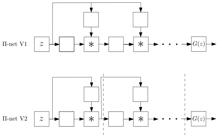
Figure 1: In this paper we introduce a class of networks called $\Pi-$ nets, where the output is a polynomial of the input. The input in this case, $_{z}$ , can be either the latent space of Generative Adversarial Network for a generative task or an image in the case of a discriminative task. Our polynomial networks can be easily implemented using a special kind of skip connections.
图 1: 本文介绍了一类称为$\Pi-$网络的结构,其输出是输入的多项式。此处的输入$_{z}$可以是生成式对抗网络(Generative Adversarial Network)在生成任务中的隐空间,也可以是判别任务中的图像。我们的多项式网络可通过一种特殊的跳跃连接(skip connections)轻松实现。
DCNNs have been used in computer vision for over 30 years [33, 50]. Arguably, what brought DCNNs again in mainstream research was the remarkable results achieved by the so-called AlexNet in the ImageNet challenge [32]. Even though it is only seven years from this pioneering effort the field has witnessed dramatic improvement in all datadependent tasks, such as object detection [21] and image generation [37, 15], just to name a few examples. The improvement is mainly attributed to carefully selected units in the architectural pipeline of DCNNs, such as blocks with skip connections [17], sophisticated normalization schemes (e.g., batch normalisation [23]), as well as the use of efficient gradient-based optimization techniques [28].
深度卷积神经网络 (DCNNs) 在计算机视觉领域已有超过 30 年的应用历史 [33, 50]。可以说,让 DCNNs 重新成为主流研究的契机是 AlexNet 在 ImageNet 挑战赛中取得的突破性成果 [32]。尽管距离这一开创性工作仅过去七年,该领域已在所有依赖数据的任务中取得了显著进步,例如目标检测 [21] 和图像生成 [37, 15] 等。这些进步主要归功于对 DCNN 架构流程中组件的精心选择,例如带有跳跃连接 (skip connections) 的模块 [17]、复杂的归一化方案(如批量归一化 [23]),以及高效梯度优化技术 [28] 的应用。
Parallel to the development of DCNN architectures for disc rim i native tasks, such as classification, the notion of Generative Adversarial Networks (GANs) was introduced for training generative models. GANs became instantly a popular line of research but it was only after the careful design of DCNN pipelines and training strategies that GANs were able to produce realistic images [26, 2]. ProGAN [25] was the first architecture to synthesize realistic facial images by a DCNN. StyleGAN [26] is a follow-up work that improved ProGAN. The main addition of StyleGAN was a type of skip connections, called ADAIN [22], which allowed the latent representation to be infused in all different layers of the generator. Similar infusions were introduced in [42] for conditional image generation.
在开发用于分类等判别任务的DCNN架构的同时,生成对抗网络(GAN)的概念被提出用于训练生成模型。GAN迅速成为热门研究方向,但只有在精心设计DCNN流程和训练策略后,GAN才能生成逼真图像[26, 2]。ProGAN[25]是首个通过DCNN合成逼真人脸图像的架构。StyleGAN[26]作为后续研究改进了ProGAN,其主要创新是一种称为ADAIN[22]的跳跃连接,允许潜在表征注入生成器的所有不同层。文献[42]针对条件图像生成提出了类似的注入机制。
Our work is motivated by the improvement of StyleGAN over ProGAN by such a simple infusion layer and the need to provide an explanation 1. We show that such infusion layers create a special non-linear structure, i.e., a higher-order polynomial, which empirically improves the representation power of DCNNs. We show that this infusion layer can be generalized (e.g. see Fig. 1) and applied in various ways in both generative, as well as disc rim i native architectures. In particular, the paper bears the following contributions:
我们的研究灵感源于StyleGAN通过简单注入层对ProGAN的改进以及解释需求[1]。我们证明这类注入层会形成特殊的非线性结构(即高阶多项式),实验表明其能提升深度卷积神经网络(DCNNs)的表征能力。如图1所示,这种注入层具有可泛化性,可灵活应用于生成式与判别式架构。本文具体贡献包括:
• We propose a new family of neural networks (called Π´nets) where the output is a high-order polynomial of the input. To avoid the combinatorial explosion in the number of parameters of polynomial activation functions [27] our Π´nets use a special kind of skip connections to implement the polynomial expansion (please see Fig. 1 for a brief schematic representation). We theoretically demonstrate that these kind of skip connections relate to special forms of tensor decompositions. • We show how the proposed architectures can be applied in generative models such as GANs, as well as disc rim i native networks. We showcase that the resulting architectures can be used to learn high-dimensional distributions without non-linear activation functions. • We convert state-of-the-art baselines using the proposed
• 我们提出了一种新型神经网络家族(称为Π´nets),其输出是输入的高阶多项式。为避免多项式激活函数参数数量的组合爆炸[27],我们的Π´nets采用特殊跳跃连接来实现多项式展开(简要示意图见图1)。我们从理论上证明这类跳跃连接与特定形式的张量分解相关。
• 我们展示了所提架构如何应用于生成式模型(如GAN)和判别式网络。实验证明该架构无需非线性激活函数即可学习高维分布。
• 我们将现有先进基线模型转换为...
Π´nets and show how they can largely improve the expressivity of the baseline. We demonstrate it conclusively in a battery of tasks (i.e., generation and classification). Finally, we demonstrate that our architectures are applicable to many different signals such as images, meshes, and audio.
Π´nets 并展示它们如何大幅提升基线的表达能力。我们通过一系列任务(即生成和分类)进行了充分验证。最后,我们证明了该架构可适用于图像、网格和音频等多种信号。
2. Related work
2. 相关工作
Expressivity of (deep) neural networks: The last few years, (deep) neural networks have been applied to a wide range of applications with impressive results. The performance boost can be attributed to a host of factors including: a) the availability of massive datasets [4, 35], b) the machine learning libraries [57, 43] running on massively parallel hardware, c) training improvements. The training improvements include a) optimizer improvement [28, 46], b) augmented capacity of the network [53], c) regular iz ation tricks [11, 49, 23, 58]. However, the paradigm for each layer remains largely unchanged for several decades: each layer is composed of a linear transformation and an element-wise activation function. Despite the variety of linear transformations [9, 33, 32] and activation functions [44, 39] being used, the effort to extend this paradigm has not drawn much attention to date.
(深度)神经网络的表达能力:过去几年,(深度)神经网络已在众多领域展现出惊人性能。这种提升可归因于以下因素:a) 海量数据集[4,35]的可用性;b) 基于大规模并行硬件的机器学习库[57,43];c) 训练优化技术。训练优化具体包括:a) 优化器改进[28,46];b) 网络容量增强[53];c) 正则化技巧[11,49,23,58]。但数十年来,每层网络的底层范式基本未变:均由线性变换和逐元素激活函数构成。尽管存在多种线性变换[9,33,32]和激活函数[44,39]方案,突破该范式的尝试至今仍未引起足够重视。
Recently, hierarchical models have exhibited stellar performance in learning expressive generative models [2, 26, 70]. For instance, the recent BigGAN [2] performs a hierarchical composition through skip connections from the noise $_{z}$ to multiple resolutions of the generator. A similar idea emerged in StyleGAN [26], which is an improvement over the Progressive Growing of GANs (ProGAN) [25]. As ProGAN, StyleGAN is a highly-engineered network that achieves compelling results on synthesized 2D images. In order to provide an explanation on the improvements of StyleGAN over ProGAN, the authors adopt arguments from the style transfer literature [22]. We believe that these improvements can be better explained under the light of our proposed polynomial function approximation. Despite the hierarchical composition proposed in these works, we present an intuitive and mathematically elaborate method to achieve a more precise approximation with a polynomial expansion. We also demonstrate that such a polynomial expansion can be used in both image generation (as in [26, 2]), image classification, and graph representation learning.
最近,分层模型在学习表达性生成模型方面展现出卓越性能[2, 26, 70]。例如,最新的BigGAN[2]通过从噪声$_{z}$到生成器多分辨率的跳跃连接实现分层组合。类似思想出现在StyleGAN[26]中,这是对渐进增长GAN(ProGAN)[25]的改进。与ProGAN一样,StyleGAN是经过高度工程化的网络,在合成2D图像上取得了令人信服的结果。为了解释StyleGAN相对ProGAN的改进,作者采用了风格迁移文献[22]中的论点。我们认为这些改进可以通过我们提出的多项式函数近似得到更好解释。尽管这些工作提出了分层组合方法,但我们提出了一种直观且数学严谨的多项式展开方法来实现更精确的近似。我们还证明这种多项式展开可同时应用于图像生成(如[26, 2])、图像分类和图表示学习。
Polynomial networks: Polynomial relationships have been investigated in two specific categories of networks: a) self-organizing networks with hard-coded feature selection, b) pi-sigma networks.
多项式网络:多项式关系已在两类特定网络中被研究:a) 具有硬编码特征选择的自组织网络,b) Pi-Sigma网络。
The idea of learnable polynomial features can be traced back to Group Method of Data Handling (GMDH) $[24]^{2}$ . GMDH learns partial descriptors that capture quadratic correlations between two predefined input elements. In [41], more input elements are allowed, while higher-order polynomials are used. The input to each partial descriptor is predefined (subset of the input elements), which does not allow the method to scale to high-dimensional data with complex correlations.
可学习多项式特征的思想可以追溯到数据处理分组方法 (GMDH) [24]^2。GMDH通过学习部分描述符来捕捉两个预定义输入元素之间的二次相关性。在[41]中,该方法允许更多输入元素,同时使用更高阶多项式。每个部分描述符的输入都是预定义的(输入元素的子集),这使得该方法无法扩展到具有复杂相关性的高维数据。
Shin et al. [51] introduce the pi-sigma network, which is a neural network with a single hidden layer. Multiple affine transformations of the data are learned; a product unit multiplies all the features to obtain the output. Improvements in the pi-sigma network include regular iz ation for training in [66] or using multiple product units to obtain the output in [61]. The pi-sigma network is extended in sigma-pi-sigma neural network (SPSNN) [34]. The idea of SPSNN relies on summing different pi-sigma networks to obtain each output. SPSNN also uses a predefined basis (overlapping rectangular pulses) on each pi-sigma sub-network to filter the input features. Even though such networks use polynomial features or products, they do not scale well in high-dimensional signals. In addition, their experimental evaluation is conducted only on signals with known ground-truth distributions (and with up to 3 dimensional input/output), unlike the modern generative models where only a finite number of samples from high-dimensional ground-truth distributions is available.
Shin等人[51]提出了pi-sigma网络,这是一种具有单隐藏层的神经网络。该网络学习数据的多重仿射变换,通过乘积单元将所有特征相乘获得输出。针对pi-sigma网络的改进包括文献[66]提出的训练正则化方法,以及文献[61]采用多重乘积单元获取输出的方案。该网络在sigma-pi-sigma神经网络(SPSNN)[34]中得到扩展,其核心思想是通过叠加不同pi-sigma网络来获得每个输出。SPSNN还在每个pi-sigma子网络中使用预定义基函数(重叠矩形脉冲)来过滤输入特征。尽管这类网络采用了多项式特征或乘积运算,但在高维信号中扩展性不佳。此外,其实验评估仅针对已知真实分布的信号(且输入/输出维度不超过3维),这与现代生成模型形成对比——后者仅需从高维真实分布中获取有限样本即可工作。
3. Method
3. 方法
Notation: Tensors are symbolized by calligraphic letters, e.g., ${x}$ , while matrices (vectors) are denoted by uppercase (lowercase) boldface letters e.g., $\ensuremath{\boldsymbol{X}},(\ensuremath{\boldsymbol{x}})$ . The mode-m vector product of ${x}$ with a vector $\pmb{u}\in\mathbb{R}^{I_{m}}$ is denoted by $\pmb{x}\times_{m}\pmb{u}$ .3
符号说明:张量 (tensor) 用花体字母表示,例如 ${x}$,矩阵 (matrix) 用大写粗体字母表示 (如 $\ensuremath{\boldsymbol{X}}$),向量 (vector) 用小写粗体字母表示 (如 $\ensuremath{\boldsymbol{x}}$)。张量 ${x}$ 与向量 $\pmb{u}\in\mathbb{R}^{I_{m}}$ 的模-m向量积记为 $\pmb{x}\times_{m}\pmb{u}$。
We want to learn a function approx im at or where each element of the output $x_{j}$ , with $j\in[1,o]$ , is expressed as a polynomial 4 of all the input elements $z_{i}$ , with $i\in[1,d]$ . That is, we want to learn a function $G:\mathbb{R}^{d}\rightarrow\mathbb{R}^{o}$ of order $N\in\mathbb N$ , such that:
我们想要学习一个函数近似器,其中输出的每个元素 $x_{j}$($j\in[1,o]$)表示为所有输入元素 $z_{i}$($i\in[1,d]$)的多项式。也就是说,我们希望学习一个阶数为 $N\in\mathbb N$ 的函数 $G:\mathbb{R}^{d}\rightarrow\mathbb{R}^{o}$,满足:
$$
\begin{array}{r}{x_{j}=G(z){j}=\beta_{j}+\pmb{w}{j}^{[1]^{T}}z+z^{T}\pmb{W}{j}^{[2]}z+}\ {\pmb{w}{j}^{[3]}\times_{1}z\times_{2}z\times_{3}z+\cdot\cdot..+\pmb{\mathscr{W}}{j}^{[N]}\displaystyle\prod_{n=1}^{N}\times_{n}z}\end{array}
$$
$$
\begin{array}{r}{x_{j}=G(z){j}=\beta_{j}+\pmb{w}{j}^{[1]^{T}}z+z^{T}\pmb{W}{j}^{[2]}z+}\ {\pmb{w}{j}^{[3]}\times_{1}z\times_{2}z\times_{3}z+\cdot\cdot..+\pmb{\mathscr{W}}{j}^{[N]}\displaystyle\prod_{n=1}^{N}\times_{n}z}\end{array}
$$
where βj P R, and Wrjns P Rśnm“1 ˆmd N are parameters for approximating the output $x_{j}$ . The correlations (of the input elements $z_{i}$ ) up to $N^{t{\bar{h}}}$ order emerge in (1). A more compact expression of (1) is obtained by vector i zing the outputs:
其中βj ∈ R,Wrjns ∈ Rśnm“1 ˆmd N 是用于逼近输出$x_{j}$的参数。(1)式中出现了输入元素$z_{i}$最高至$N^{t{\bar{h}}}$阶的相关性。通过向量化输出可以得到(1)式更简洁的表达式:
$$
\pmb{x}=G(z)=\sum_{n=1}^{N}\left(\pmb{\mathcal{W}}^{[n]}\prod_{j=2}^{n+1}\times_{j}z\right)+\beta
$$
$$
\pmb{x}=G(z)=\sum_{n=1}^{N}\left(\pmb{\mathcal{W}}^{[n]}\prod_{j=2}^{n+1}\times_{j}z\right)+\beta
$$
where β P Ro and Wrns P Roˆśnm“1 ˆmd N are the learnable parameters. This form of (2) allows us to approximate any smooth function (for large $N$ ), however the parameters grow with $\mathcal{O}(d^{N})$ .
其中β ∈ ℝ^o和W_rns ∈ ℝ^{o×∏_{m=1}^N d_m}是可学习参数。这种形式的(2)允许我们逼近任何光滑函数(对于较大的$N$),但参数会以$\mathcal{O}(d^{N})$的复杂度增长。
A variety of methods, such as pruning [8, 16], tensor decomposition s [29, 52], special linear operators [6] with reduced parameters, parameter sharing/prediction [67, 5], can be employed to reduce the parameters. In contrast to the heuristic approaches of pruning or prediction, we describe below two principled ways which allow an efficient implementation. The first method relies on performing an off-the-shelf tensor decomposition on (2), while the second considers the final polynomial as the product of lower-degree polynomials.
可以采用多种方法来减少参数,例如剪枝 [8, 16]、张量分解 [29, 52]、参数减少的特殊线性算子 [6]、参数共享/预测 [67, 5]。与剪枝或预测的启发式方法不同,我们下面描述两种允许高效实现的原则性方法。第一种方法依赖于对(2)执行现成的张量分解,而第二种方法将最终多项式视为低次多项式的乘积。
The tensor decomposition s are used in this paper to provide a theoretical understanding (i.e., what is the order of the polynomial used) of the proposed family of Π-nets. Implementation-wise the incorporation of different $\Pi$ -net structures is as simple as the in corpora t ation of a skipconnection. Nevertheless, in $\Pi$ -net different skip connections lead to different kinds of polynomial networks.
本文使用张量分解 (tensor decomposition) 为提出的Π网络家族提供理论解释 (即所用多项式的阶数)。在实现层面,集成不同$\Pi$网络结构的操作如同添加跳跃连接 (skip connection) 一样简单。然而在$\Pi$网络中,不同的跳跃连接会生成不同类型的多项式网络。
3.1. Single polynomial
3.1. 单多项式
A tensor decomposition on the parameters is a natural way to reduce the parameters and to implement (2) with a neural network. Below, we demonstrate how three such decomposition s result in novel architectures for a neural network training. The main symbols are summarized in Table 1, while the equivalence between the recursive relationship and the polynomial is analyzed in the supplementary.
对参数进行张量分解是减少参数并用神经网络实现(2)的自然方法。下面我们将展示三种此类分解如何产生新颖的神经网络训练架构。主要符号汇总在表1中,而递归关系与多项式之间的等价性分析详见补充材料。
Model 1: CCP: A coupled CP decomposition [29] is applied on the parameter tensors. That is, each parameter tensor, i.e. $w^{[\dot{n}]}$ for $n\in[1,N]$ , is not factorized individually, but rather a coupled factorization of the parameters is defined. The recursive relationship is:
模型1: CCP: 对参数张量采用耦合CP分解[29]。即每个参数张量(如$w^{[\dot{n}]}$, $n\in[1,N]$)不再单独分解,而是定义参数的耦合分解。其递推关系为:
$$
\pmb{x}{n}=\left(U_{[n]}^{T}z\right)\ast\pmb{x}{n-1}+\pmb{x}_{n-1}
$$
$$
\pmb{x}{n}=\left(U_{[n]}^{T}z\right)\ast\pmb{x}{n-1}+\pmb{x}_{n-1}
$$
for $n=2,\ldots,N$ with $x_{1}=U_{[1]}^{T}z$ and ${\pmb x}={\pmb C}{\pmb x}{N}+\beta$ The parameters $C\in\mathbb{R}^{o\times k},\pmb{U}_{[n]}\bar{\in\mathbb{R}}^{d\times k}$ for $n=1,\ldots,N$ are learnable. To avoid overloading the diagram, a schematic assuming a third order expansion $N=3,$ ) is illustrated in Fig. 2.
对于 $n=2,\ldots,N$,其中 $x_{1}=U_{[1]}^{T}z$ 且 ${\pmb x}={\pmb C}{\pmb x}{N}+\beta$。参数 $C\in\mathbb{R}^{o\times k},\pmb{U}_{[n]}\bar{\in\mathbb{R}}^{d\times k}$($n=1,\ldots,N$)是可学习的。为避免图示过载,图 2 展示了三阶展开 $N=3$ 的示意图。
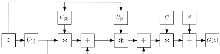
Figure 2: Schematic illustration of the CCP (for third order approximation). Symbol $^*$ refers to the Hadamard product.
图 2: CCP(三阶近似)示意图。符号 $^*$ 表示哈达玛积(Hadamard product)。
Model 2: NCP: Instead of defining a flat CP decomposition, we can utilize a joint hierarchical decomposition on the polynomial parameters. A nested coupled CP decomposition (NCP), which results in the following recursive relationship for $N^{t h}$ order approximation is defined:
模型2:NCP:不同于定义平坦的CP分解,我们可以对多项式参数采用联合层次分解。嵌套耦合CP分解(NCP)由此产生,其第N阶近似遵循以下递归关系:
Table 1: Nomenclature
表 1: 术语表
| 符号 | 维度 | 定义 |
|---|---|---|
| n, N k 之 | N N Rd | 多项式项阶数、总逼近阶数。分解的秩。多项式逼近器(即生成器)的输入。 |
$$
\pmb{x}{n}=\left(\pmb{A}{[n]}^{T}\pmb{z}\right)*\left(\pmb{S}{[n]}^{T}\pmb{x}{n-1}+\pmb{B}{[n]}^{T}\pmb{b}_{[n]}\right)
$$
$$
\pmb{x}{n}=\left(\pmb{A}{[n]}^{T}\pmb{z}\right)*\left(\pmb{S}{[n]}^{T}\pmb{x}{n-1}+\pmb{B}{[n]}^{T}\pmb{b}_{[n]}\right)
$$
for $n=2,\ldots,N$ with $\pmb{x}{1}=\left({\pmb A}{[n]}^{T}{\pmb z}\right)*\left({\pmb B}{[n]}^{T}{\pmb b}{[n]}\right)$ and ${\pmb x}={\pmb C}{\pmb x}{N}+\beta$ . The parameters $C\in\mathbb{R}^{o\times k},A_{[n]}\in$ $\mathbb{R}^{d\times k},S_{[n]}\in\mathbb{R}^{k\times k},B_{[n]}\in\mathbb{R}^{\omega\times k}$ , $b_{[n]} \in~\mathbb{R}^{\omega}$ for $n=$ $1,\ldots,N$ , are learnable. The explanation of each variable is elaborated in the supplementary, where the decomposition is derived.
对于 $n=2,\ldots,N$,其中 $\pmb{x}{1}=\left({\pmb A}{[n]}^{T}{\pmb z}\right)*\left({\pmb B}{[n]}^{T}{\pmb b}{[n]}\right)$ 且 ${\pmb x}={\pmb C}{\pmb x}{N}+\beta$。参数 $C\in\mathbb{R}^{o\times k},A_{[n]}\in$ $\mathbb{R}^{d\times k},S_{[n]}\in\mathbb{R}^{k\times k},B_{[n]}\in\mathbb{R}^{\omega\times k}$,$b_{[n]}\in~\mathbb{R}^{\omega}$ 对于 $n=$ $1,\ldots,N$ 是可学习的。各变量的详细解释及分解推导见补充材料。
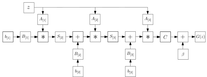
Figure 3: Schematic illustration of the NCP (for third order approximation). Symbol $^*$ refers to the Hadamard product.
图 3: NCP (三阶近似) 示意图。符号 $^*$ 表示 Hadamard 积。
Model 3: NCP-Skip: The expressiveness of NCP can be further extended using a skip connection (motivated by CCP). The new model uses a nested coupled decomposition and has the following recursive expression:
模型 3: NCP-Skip: 通过引入跳跃连接 (受CCP启发) 可进一步扩展NCP的表达能力。该新模型采用嵌套耦合分解,其递归表达式如下:
$$
\pmb{x}{n}=\left(\pmb{A}{[n]}^{T}\pmb{z}\right)\ast\left(\pmb{S}{[n]}^{T}\pmb{x}{n-1}+\pmb{B}{[n]}^{T}\pmb{b}{[n]}\right)+\pmb{x}_{n-1}
$$
$$
\pmb{x}{n}=\left(\pmb{A}{[n]}^{T}\pmb{z}\right)\ast\left(\pmb{S}{[n]}^{T}\pmb{x}{n-1}+\pmb{B}{[n]}^{T}\pmb{b}{[n]}\right)+\pmb{x}_{n-1}
$$
for $n=2,\ldots,N$ with $\pmb{x}{1}=\left(\pmb{A}{[n]}^{T}\pmb{z}\right)\ast\left(\pmb{B}{[n]}^{T}\pmb{b}{[n]}\right)$ and ${\pmb x}={\pmb C}{\pmb x}_{N}+\beta$ . The learnable parameters are the same as in NCP, however the difference in the recursive form results in a different polynomial expansion and thus architecture.
对于 $n=2,\ldots,N$,其中 $\pmb{x}{1}=\left(\pmb{A}{[n]}^{T}\pmb{z}\right)\ast\left(\pmb{B}{[n]}^{T}\pmb{b}{[n]}\right)$ 且 ${\pmb x}={\pmb C}{\pmb x}_{N}+\beta$。可学习参数与NCP相同,但递归形式的不同导致了多项式展开的差异,从而形成了不同的架构。
Comparison between the models: All three models are based on a polynomial expansion, however their recursive forms and employed decomposition s differ. The CCP has a simpler expression, however the NCP and the NCP-Skip relate to standard architectures using hierarchical composition that have recently yielded promising results in both generative and disc rim i native tasks. In the remainder of the paper, for comparison purposes we use the NCP by default for the image generation and NCP-Skip for the image classification. In our preliminary experiments, CCP and NCP share a similar performance based on the setting of Sec. 4. In all cases, to mitigate stability issues that might emerge during training, we employ certain normalization schemes that constrain the magnitude of the gradients. An in-depth theoretical analysis of the architectures is deferred to a future version of our work.
模型对比:
这三种模型均基于多项式展开,但它们的递归形式与所采用的分解方法各不相同。CCP表达式较为简洁,而NCP和NCP-Skip则关联到采用分层组合的标准架构,这些架构近期在生成式和判别式任务中均展现出良好效果。本文后续部分默认使用NCP进行图像生成实验,NCP-Skip用于图像分类实验以便对比。初步实验中,CCP与NCP在第四节设定下表现相近。所有实验均采用特定归一化方案约束梯度幅度,以缓解训练中可能出现的稳定性问题。架构的深度理论分析将留待后续工作版本探讨。
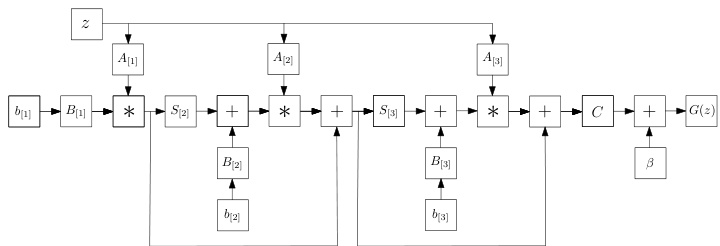
Figure 4: Schematic illustration of the NCP-Skip (for third order approximation). The difference from Fig. 3 is the skip connections added in this model.
图 4: NCP-Skip示意图(三阶近似)。与图3的区别在于该模型增加了跳跃连接。
3.2. Product of polynomials
3.2. 多项式乘积
Instead of using a single polynomial, we express the function approximation as a product of polynomials. The product is implemented as successive polynomials where the output of the $i^{t h}$ polynomial is used as the input for the $(i+1)^{t h}$ polynomial. The concept is visually depicted in Fig. 5; each polynomial expresses a second order expansion. Stacking $N$ such polynomials results in an overall order of $2^{N}$ . Trivially, if the approximation of each polynomial is $B$ and we stack $N$ such polynomials, the total order is $B^{N}$ . The product does not necessarily demand the same order in each polynomial, the expressivity and the expansion order of each polynomial can be different and dependent on the task, e.g. for generative tasks that the resolution increases progressively, the expansion order could increase in the last polynomials. In all cases, the final order will be the product of each polynomial.
我们不使用单一多项式,而是将函数近似表示为多项式的乘积。该乘积通过连续多项式实现,其中第$i^{t h}$个多项式的输出作为第$(i+1)^{t h}$个多项式的输入。这一概念在图5中直观展示:每个多项式表示二阶展开。堆叠$N$个这样的多项式将获得$2^{N}$阶的整体展开度。显然,若每个多项式的近似阶数为$B$且堆叠$N$个多项式,则总阶数为$B^{N}$。乘积中的多项式不必具有相同阶数,每个多项式的表达能力和展开阶数可因任务而异,例如在分辨率逐步提升的生成式任务中,最后几个多项式的展开阶数可递增。所有情况下,最终阶数均为各多项式阶数的乘积。
There are two main benefits of the product over the single polynomial: a) it allows using different decomposition s (e.g. like in Sec. 3.1) and expressive power for each polynomial; b) it requires much less parameters for achieving the same order of approximation. Given the benefits of the product of polynomials, we assume below that a product of polynomials is used, unless explicitly mentioned otherwise. The respective model of product polynomials is called ProdPoly.
该产品相较于单一多项式主要有两大优势:
a) 允许为每个多项式采用不同的分解方式(如第3.1节所述)和表达能力;
b) 在达到相同逼近阶数时所需参数大幅减少。鉴于多项式乘积的优越性,下文默认采用多项式乘积模型(除非另有说明),该模型称为ProdPoly。
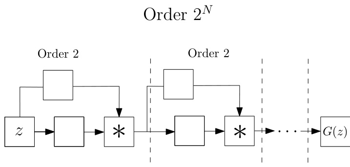
Figure 5: Abstract illustration of the ProdPoly. The input variable $_{z}$ on the left is the input to a $2^{n d}$ order expansion; the output of this is used as the input for the next polynomial (also with a $2^{n d}$ order expansion) and so on. If we use $N$ such polynomials, the final output $G(z)$ expresses a $2^{N}$ order expansion. In addition to the high order of approximation, the benefit of using the product of polynomials is that the model is flexible, in the sense that each polynomial can be implemented as a different decomposition of Sec. 3.1.
图 5: ProdPoly的抽象示意图。左侧输入变量 $_{z}$ 作为 $2^{n d}$ 阶展开的输入;其输出又作为下一个多项式(同样采用 $2^{n d}$ 阶展开)的输入,依此类推。若使用 $N$ 个这样的多项式,最终输出 $G(z)$ 将呈现 $2^{N}$ 阶展开。除了高阶近似能力外,采用多项式乘积的优势在于模型具有灵活性——每个多项式均可实现为第3.1节所述的不同分解形式。
3.3. Task-dependent input/output
3.3. 任务相关的输入/输出
The aforementioned polynomials are a function $\textbf{{x}}=$ $G(z)$ , where the input/output are task-dependent. For a generative task, e.g. learning a decoder, the input ${z}$ is typically some low-dimensional noise, while the output is a high-dimensional signal, e.g. an image. For a disc rim i native task the input ${z}$ is an image; for a domain adaptation task the signal ${z}$ denotes the source domain and $_{x}$ the target domain.
上述多项式是函数 $\textbf{{x}}=$ $G(z)$,其输入/输出取决于具体任务。对于生成式任务(例如学习解码器),输入 ${z}$ 通常是低维噪声,而输出是高维信号(如图像)。对于判别任务,输入 ${z}$ 是图像;对于域适应任务,信号 ${z}$ 表示源域,而 $_{x}$ 表示目标域。
4. Proof of concept
4. 概念验证
In this Section, we conduct motivational experiments in both generative and disc rim i native tasks to demonstrate the expressivity of Π´nets. Specifically, the networks are implemented without activation functions, i.e. only linear operations (e.g. convolutions) and Hadamard products are used. In this setting, the output is linear or multi-linear with respect to the parameters.
在本节中,我们在生成式和判别式任务中进行了动机实验,以证明Π´nets的表达能力。具体而言,这些网络在没有激活函数的情况下实现,即仅使用线性操作(如卷积)和Hadamard积。在此设置下,输出相对于参数是线性或多线性的。
4.1. Linear generation
4.1. 线性生成
One of the most popular generative models is Generative Adversarial Nets (GAN) [12]. We design a GAN, where the generator is implemented as a product of polynomials (using the NCP decomposition), while the disc rim in at or of [37] is used. No activation functions are used in the generator, but a single hyperbolic tangent (tanh) in the image space 5.
最流行的生成模型之一是生成对抗网络 (GAN) [12]。我们设计了一个GAN,其中生成器实现为多项式乘积 (使用NCP分解),而判别器采用[37]的方案。生成器中没有使用激活函数,但在图像空间5中使用了单个双曲正切 (tanh)。
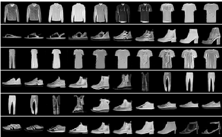
Figure 6: Linear interpolation in the latent space of ProdPoly (when trained on fashion images [64]). Note that the generator does not include any activation functions in between the linear blocks (Sec. 4.1). All the images are synthesized; the image on the leftmost column is the source, while the one in the rightmost is the target synthesized image.
图 6: ProdPoly (在时尚图像 [64] 上训练时) 潜在空间中的线性插值。注意生成器在线性块之间不包含任何激活函数 (第 4.1 节)。所有图像均为合成图像;最左侧列图像为源图像,最右侧列图像为目标合成图像。
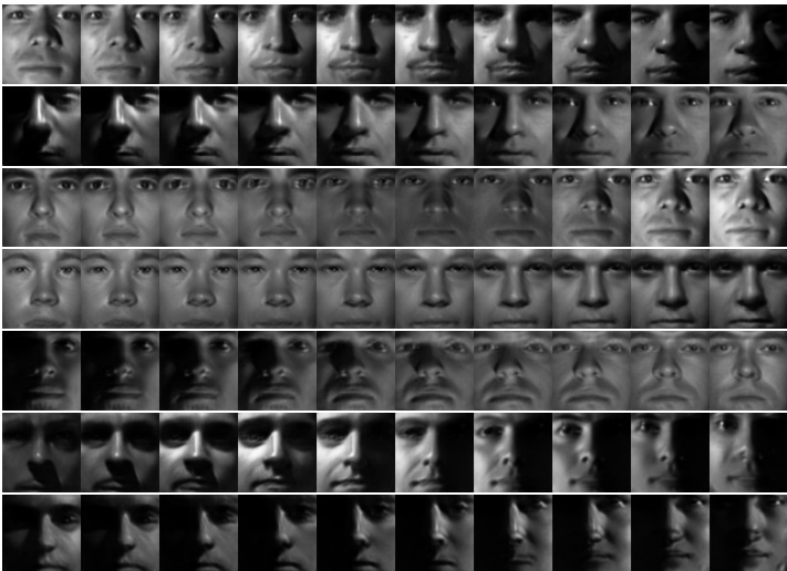
Figure 7: Linear interpolation in the latent space of ProdPoly (when trained on facial images [10]). As in Fig. 6, the generator includes only linear blocks; the image on the leftmost column is the source, while the one in the rightmost is the target image.
图 7: ProdPoly 潜在空间中的线性插值 (在面部图像上训练时 [10])。与图 6 相同,生成器仅包含线性块;最左侧列中的图像是源图像,而最右侧列中的是目标图像。
Two experiments are conducted with a polynomial generator (Fashion-Mnist and YaleB). We perform a linear inter pol ation in the latent space when trained with FashionMnist [64] and with YaleB [10] and visualize the results in Figs. 6, 7, respectively. Note that the linear interpolation generates plausible images and navigates among different categories, e.g. trousers to sneakers or trousers to t-shirts. Equivalently, it can linearly traverse the latent space from a fully illuminated to a partly dark face.
我们使用多项式生成器进行了两项实验(Fashion-Mnist和YaleB)。在FashionMnist [64]和YaleB [10]训练时,我们在潜在空间进行线性插值,并分别在 图 6 和图 7 中可视化结果。值得注意的是,线性插值生成了合理的图像,并在不同类别之间进行转换,例如从裤子到运动鞋或从裤子到T恤。同样地,它可以在潜在空间中从完全明亮的面部线性过渡到部分阴暗的面部。
4.2. Linear classification
4.2. 线性分类
To empirically illustrate the power of the polynomial, we use ResNet without activation s for classification. Residual Network (ResNet) [17, 54] and its variants [21, 62, 65, 69,
为了实证说明多项式的强大能力,我们使用不带激活函数的ResNet进行分类。残差网络(ResNet) [17, 54]及其变体[21, 62, 65, 69,

Figure 8: Image classification accuracy with linear residual blocks6. The schematic on the left is on CIFAR10 classification, while the one on the right is on CIFAR100 classification.
图 8: 使用线性残差块 (linear residual blocks) 的图像分类准确率6。左侧示意图展示 CIFAR10 分类结果,右侧为 CIFAR100 分类结果。
68] have been applied to diverse tasks including object detection and image generation [14, 15, 37]. The core component of ResNet is the residual block; the $t^{t h}$ residual block is expressed as $z_{t+1}=z_{t}+C z_{t}$ for input $z_{t}$ .
68] 已被应用于包括目标检测和图像生成在内的多种任务 [14, 15, 37]。ResNet的核心组件是残差块 (residual block);第 $t^{t h}$ 个残差块的输入 $z_{t}$ 可表示为 $z_{t+1}=z_{t}+C z_{t}$。
We modify each residual block to express a higher order interaction, which can be achieved with NCP-Skip. The output of each residual block is the input for the next residual block, which makes our ResNet a product of polynomials. We conduct a classification experiment with CIFAR10 [31] (10 classes) and CIFAR100 [30] (100 classes). Each residual block is modified in two ways: a) all the activation functions are removed, b) it is converted into an $i^{t h}$ order expansion with $i\in[2,5]$ . The second order expansion (for the $t^{t h}$ residual block) is expressed as $z_{t+1}=z_{t}+C z_{t}+\left(C z_{t}\right)$ $z_{t}$ ; higher orders are constructed similarly by performing a Hadamard product of the last term with $z_{t}$ (e.g., for third order expansion it would be $z_{t+1}=z_{t}+C z_{t}+\left(C z_{t}\right)*$ $z_{t}+\left(C z_{t}\right)*z_{t}*z_{t})$ . The following two variations are evaluated: a) a single residual block is used in each ‘group layer’, b) two blocks are used per ‘group layer’. The latter variation is equivalent to ResNet18 without activation s.
我们对每个残差块进行修改,以表达更高阶的交互,这可以通过NCP-Skip实现。每个残差块的输出作为下一个残差块的输入,使得我们的ResNet成为多项式乘积。我们在CIFAR10 [31](10类)和CIFAR100 [30](100类)上进行了分类实验。每个残差块通过两种方式修改:a) 移除所有激活函数,b) 将其转换为$i^{th}$阶扩展,其中$i\in[2,5]$。二阶扩展(针对第$t^{th}$个残差块)表示为$z_{t+1}=z_{t}+C z_{t}+\left(C z_{t}\right)$$z_{t}$;更高阶扩展通过将最后一项与$z_{t}$进行Hadamard乘积来构造(例如,三阶扩展为$z_{t+1}=z_{t}+C z_{t}+\left(C z_{t}\right)*$$z_{t}+\left(C z_{t}\right)*z_{t}*z_{t})$。评估了以下两种变体:a) 每个“组层”使用单个残差块,b) 每个“组层”使用两个块。后一种变体相当于不带激活函数的ResNet18。
Each experiment is conducted 10 times; the mean accuracy is reported in Fig. 8. We note that the same trends emerge in both datasets6. The performance remains similar irrespective of the the amount of residual blocks in the group layer. The performance is affected by the order of the expansion, i.e. higher orders cause a decrease in the accuracy. Our conjecture is that this can be partially attributed to over fitting (note that a $3^{r d}$ order expansion for the 2222 block - in total 8 res. units - yields a polynomial of $3^{8}$ power), however we defer a detailed study of this in a future version of our work. Nevertheless, in all cases without activation s the accuracy is close to the original ResNet18 with activation functions.
每个实验进行10次;平均准确率如图8所示。我们注意到两个数据集6都呈现相同趋势。无论分组层中包含多少残差块(residual blocks),性能都保持相似。性能受扩展阶数影响,即更高阶数会导致准确率下降。我们推测这可能部分归因于过拟合(注意2222模块的3阶扩展——共8个残差单元——会产生3的8次方多项式),但详细研究将留待后续工作版本。不过在所有未使用激活函数的案例中,准确率都接近带激活函数的原始ResNet18。
Table 2: IS/FID scores on CIFAR10 [31] generation. The scores of [14, 15] are added from the respective papers as using similar residual based generators. The scores of [7, 19, 36] represent alternative generative models. Prod Poly outperform the compared methods in both metrics.
表 2: CIFAR10 [31] 生成任务的 IS/FID 分数。[14, 15] 的分数来自各自论文(使用类似的基于残差的生成器)。[7, 19, 36] 的分数代表其他生成模型。Prod Poly 在两项指标上均优于对比方法。
| 模型 | IS (↑) | FID (↓) |
|---|---|---|
| SNGAN | 8.06 ± 0.10 | 19.06 ± 0.50 |
| NCP(Sec. 3.1) | 8.30 ± 0.09 | 17.65 ± 0.76 |
| ProdPoly | 8.49 ± 0.11 | 16.79 ± 0.81 |
| CSGAN-[14] | 7.90 ± 0.09 | - |
| WGAN-GP-[15] | 7.86 ± 0.08 | - |
| CQFG-[36] | 8.10 | 18.60 |
| EBM [7] | 6.78 | 38.2 |
| GLANN [19] | - | 46.5 ± 0.20 |
5. Experiments
5. 实验
We conduct three experiments against state-of-the-art models in three diverse tasks: image generation, image classification, and graph representation learning. In each case, the baseline considered is converted into an instance of our family of $\Pi$ -nets and the two models are compared.
我们在图像生成、图像分类和图表示学习这三个多样化任务中,针对最先进的模型进行了三项实验。每种情况下,所考虑的基线模型都被转换为我们 $\Pi$ 网家族的一个实例,并对两种模型进行比较。
5.1. Image generation
5.1. 图像生成
The robustness of ProdPoly in image generation is assessed in two different architectures/datasets below.
ProdPoly在图像生成中的鲁棒性在以下两种架构/数据集中进行评估。
SNGAN on CIFAR10: In the first experiment, the architecture of SNGAN [37] is selected as a strong baseline on CIFAR10 [31]. The baseline includes 3 residual blocks in the generator and the disc rim in at or.
CIFAR10上的SNGAN:在第一个实验中,我们选择SNGAN [37]的架构作为CIFAR10 [31]上的强基线。该基线在生成器中包含3个残差块,判别器采用相同结构。
The generator is converted into a $\Pi$ -net, where each residual block is a single order of the polynomial. We implement two versions, one with a single polynomial (NCP) and one with product of polynomials (where each polynomial uses NCP). In our implementation $\pmb{A}{[n]}$ is a thin FC layer, $(B_{[n]})^{T}{\pmb b}{[n]}$ is a bias vector and $S_{[n]}$ is the transformation of the residual block. Other than the aforementioned modifications, the hyper-parameters (e.g. disc rim in at or, learning rate, optimization details) are kept the same as in [37].
生成器被转换为一个$\Pi$网络,其中每个残差块是多项式的一个单阶项。我们实现了两个版本:一个是单一多项式(NCP),另一个是多项式乘积(其中每个多项式采用NCP)。在我们的实现中,$\pmb{A}{[n]}$是一个窄的全连接层,$(B_{[n]})^{T}{\pmb b}{[n]}$是偏置向量,$S_{[n]}$表示残差块的变换。除上述修改外,超参数(例如判别器、学习率、优化细节)均与文献[37]保持一致。
Each network has run for 10 times and the mean and variance are reported. The popular Inception Score (IS) [48] and the Frechet Inception Distance (FID) [18] are used for quantitative evaluation. Both scores extract feature representations from a pre-trained classifier (the Inception network [56]).
每个网络运行10次并报告均值和方差。采用流行的Inception Score (IS) [48]和Frechet Inception Distance (FID) [18]进行定量评估。两种分数均从预训练分类器(Inception网络[56])中提取特征表示。
The quantitative results are summarized in Table 2. In addition to SNGAN and our two variations with polynomials, we have added the scores of [14, 15, 7, 19, 36] as reported in the respective papers. Note that the single polynomial already outperforms the baseline, while the ProdPoly boosts the performance further and achieves a substantial improvement over the original SNGAN.
定量结果总结在表2中。除了SNGAN和我们的两种多项式变体外,我们还添加了[14, 15, 7, 19, 36]在各自论文中报告的分数。需要注意的是,单一多项式已经超越了基线,而ProdPoly进一步提升了性能,相比原始SNGAN实现了显著改进。

Figure 9: Samples synthesized from ProdPoly (trained on FFHQ).
图 9: 基于ProdPoly (在FFHQ上训练) 生成的合成样本。
StyleGAN on FFHQ: StyleGAN [26] is the state-of-theart architecture in image generation. The generator is composed of two parts, namely: (a) the mapping network, composed of 8 FC layers, and (b) the synthesis network, which is based on ProGAN [25] and progressively learns to synthesize high quality images. The sampled noise is transformed by the mapping network and the resulting vector is then used for the synthesis network. As discussed in the introduction StyleGAN is already an instance of the $\Pi$ -net family, due to AdaIN. Specifically, the $k^{t h}$ AdaIN layer is $h_{k}=(A_{k}^{T}w)\ast n(c(h_{k-1}))$ , where $n$ is a normalization, $c$ is a convolution and $\mathbf{\nabla}{\mathbf{\overrightarrow{\mathbf{\vert~\mathbf{\nabla~}~}}}}$ is the transformed noise ${\pmb w}=M L P({\pmb z})$ (mapping network). This is equivalent to our NCP model by setting $S_{[k]}^{T}$ as the convolution operator.
FFHQ数据集上的StyleGAN:StyleGAN [26] 是当前图像生成领域的最先进架构。生成器由两部分组成:(a) 由8个全连接层构成的映射网络,(b) 基于ProGAN [25] 的合成网络,该网络通过渐进式学习合成高质量图像。采样噪声经映射网络变换后,生成的向量被用于合成网络。如引言所述,由于采用了AdaIN技术,StyleGAN本身已是$\Pi$网络家族的实例。具体而言,第$k$层AdaIN可表示为$h_{k}=(A_{k}^{T}w)\ast n(c(h_{k-1}))$,其中$n$为归一化操作,$c$为卷积运算,$\mathbf{\nabla}{\mathbf{\overrightarrow{\mathbf{\vert~\mathbf{\nabla~}~}}}}$是经映射网络${\pmb w}=MLP({\pmb z})$变换后的噪声。通过将$S_{[k]}^{T}$设为卷积算子,该形式等价于我们的NCP模型。
In this experiment we illustrate how simple modifications, using our family of products of polynomials, further improve the representation power. We make a minimal modification in the mapping network, while fixing the rest of the hyperparameters. In particular, we convert the mapping network into a polynomial (specifically a NCP), which makes the generator a product of two polynomials.
在本实验中,我们展示了如何通过使用多项式乘积系列方法进行简单修改,从而进一步提升表征能力。我们在保持其他超参数不变的情况下,对映射网络进行了最小化修改。具体而言,我们将映射网络转换为一个多项式(特别是NCP),这使得生成器成为两个多项式的乘积。
The Flickr-Faces-HQ Dataset (FFHQ) dataset [26] which includes 70, 000 images of high-resolution faces is used. All the images are resized to $256\times256$ . The best FID scores of the two methods (in $256\times256$ resolution) are 6.82 for ours and 7.15 for the original StyleGAN, respectively. That is, our method improves the results by $5%$ . Synthesized samples of our approach are visualized in Fig. 9.
我们使用了包含7万张高分辨率人脸的Flickr-Faces-HQ数据集(FFHQ) [26]。所有图像均调整为$256\times256$分辨率。两种方法在$256\times256$分辨率下的最佳FID分数分别为:我们的方法6.82,原始StyleGAN 7.15。这表明我们的方法将结果提升了$5%$。图9展示了本方法生成的样本效果。
5.2. Classification
5.2. 分类
We perform two experiments on classification: a) audio classification, b) image classification.
我们在分类任务上进行了两项实验:a) 音频分类,b) 图像分类。
Audio classification: The goal of this experiment is twofold: a) to evaluate ResNet on a distribution that differs from that of natural images, b) to validate whether higherorder blocks make the model more expressive. The core assumption is that we can increase the expressivity of our model, or equivalently we can use less residual blocks of higher-order to achieve performance similar to the baseline.
音频分类:本实验的目标有两个:a) 在不同于自然图像的分布上评估 ResNet 的性能,b) 验证高阶模块是否能增强模型表达能力。核心假设是我们可以通过增加模型表达能力(或等效地使用更少的高阶残差模块)来达到与基线相当的性能。
The performance of ResNet is evaluated on the Speech Commands dataset [63]. The dataset includes 60, 000 audio files; each audio contains a single word of a duration of one second. There are 35 different words (classes) with each word having $1,500-4,100$ recordings. Every audio file is converted into a mel-spec tr ogram of resolution $32\times32$ .
ResNet的性能在Speech Commands数据集[63]上进行了评估。该数据集包含60,000个音频文件,每个音频包含一个持续时间为1秒的单词。共有35个不同的单词(类别),每个单词有$1,500-4,100$条录音。每个音频文件被转换为分辨率为$32\times32$的梅尔频谱图。
The baseline is a ResNet34 architecture; we use secondorder residual blocks to build the Prodpoly-ResNet to match the performance of the baseline. The quantitative results are added in Table 3. The two models share the same accuracy, however Prodpoly-ResNet includes $38%$ fewer parameters. This result validates our assumption that our model is more expressive and with even fewer parameters, it can achieve the same performance.
基线采用ResNet34架构;我们使用二阶残差块构建Prodpoly-ResNet以匹配基线性能。定量结果已添加至表3。两个模型准确率相同,但Prodpoly-ResNet参数减少了38%。该结果验证了我们的假设:我们的模型表达能力更强,即使参数更少也能达到相同性能。
Table 3: Speech classification with ResNet. The accuracy of the compared methods is similar, but Prodpoly-ResNet has $38%$ fewer parameters. The symbol ‘# par’ abbreviates the number of parameters (in millions).
表 3: 基于 ResNet 的语音分类。对比方法的准确率相近,但 Prodpoly-ResNet 参数量减少了 $38%$ 。符号 '# par' 表示参数量(单位:百万)。
| 模型 | #blocks | # par | Accuracy |
|---|---|---|---|
| ResNet34 | [3,4,6,3] | 21.3 | 0.951 ± 0.002 |
| Prodpoly-ResNet | [3,3,3,2] | 13.2 | 0.951 ± 0.002 |
Image classification: We perform a large-scale classification experiment on ImageNet [47]. We choose float16 instead of float32 to achieve $3.5\times$ acceleration and reduce the GPU memory consumption by $50%$ . To stabilize the training, the second order of each residual block is normalized with a hyperbolic tangent unit. SGD with momentum 0.9, weight decay $10^{-4}$ and a mini-batch size of 1024 is used. The initial learning rate is set to 0.4 and decreased by a factor of 10 at 30, 60, and 80 epochs. Models are trained for 90 epochs from scratch, using linear warm-up of the learning rate during first five epochs according to [13]. For other batch sizes due to the limitation of GPU memory, we linearly scale the learning rate (e.g. 0.1 for batch size 256).
图像分类:我们在ImageNet [47]上进行了大规模分类实验。选择float16而非float32以实现$3.5\times$加速,并将GPU内存消耗降低$50%$。为稳定训练,每个残差块的二阶通过双曲正切单元进行归一化。采用动量0.9的SGD优化器,权重衰减$10^{-4}$,最小批次大小为1024。初始学习率设为0.4,在第30、60和80轮时以10倍系数递减。模型从零开始训练90轮,前五轮学习率按[13]采用线性预热策略。对于因GPU内存限制导致的其他批次大小,我们线性缩放学习率(例如批次大小256对应0.1)。
The Top-1 error throughout the training is visualized in Fig. 10, while the validation results are added in Table 4. For a fair comparison, we report the results from our training in both the original ResNet and Prodpoly-ResNet7. ProdpolyResNet consistently improves the performance with an extremely small increase in computational complexity and model size. Remarkably, Prodpoly-ResNet50 achieves a single-crop Top-5 validation error of $6.358%$ , exceeding ResNet50 $(6.838%)$ by $0.48%$ .
训练过程中的Top-1错误率如图10所示,验证结果则汇总在表4中。为确保公平比较,我们同时报告了原始ResNet和Prodpoly-ResNet7的训练结果。Prodpoly-ResNet在计算复杂度和模型大小仅微量增加的情况下持续提升性能。值得注意的是,Prodpoly-ResNet50实现了单次裁剪Top-5验证错误率$6.358%$,以$0.48%$的优势超越ResNet50$(6.838%)$。
5.3. 3D Mesh representation learning
5.3. 3D网格表示学习
Below, we evaluate higher order correlations in graph related tasks. We experiment with 3D deformable meshes of fixed topology [45], i.e. the connectivity of the graph $\mathcal{G}={\mathcal{V},\mathcal{E}}$ remains the same and each different shape is defined as a different signal ${x}$ on the vertices of the graph: $\pmb{x}:\mathcal{V}\rightarrow\mathbb{R}^{d}$ . As in the previous experiments, we extend a state-of-the-art operator, namely spiral convolutions [1], with the ProdPoly formulation and test our method on the task of auto encoding 3D shapes. We use the existing architecture and hyper-parameters of [1], thus showing that ProdPoly can be used as a plug-and-play operator to existing models, turning the aforementioned one into a Spiral Π-Net. Our implementation uses a product of polynomials, where each polynomial is a specific instantiation of (4): $\pmb{x}{n}=\left(\pmb{S}{[n]}^{T}\pmb{x}{n-1}\right)^{-}\ast\left(\pmb{S}{[n]}^{T}\pmb{x}{n-1}\right)^{+}+\pmb{S}{[n]}^{T}\pmb{x}{n-1},\pmb{x}=\pmb{x}{n}+\beta,$ where $\pmb{S}$ is the spiral convolution operator written in matrix form.8 We use this model (ProdPoly simple) to showcase how to increase the expressivity without adding new blocks in the architecture. This model can be also re-interpreted as a learnable polynomial activation function as in [27]. We also show the results of our complete model (ProdPoly full), where $\pmb{A}_{[n]}$ is a different spiral convolution.
下面,我们评估图相关任务中的高阶相关性。我们采用固定拓扑的3D可变形网格[45]进行实验,即图$\mathcal{G}={\mathcal{V},\mathcal{E}}$的连通性保持不变,每个不同形状被定义为图顶点上的不同信号${x}$:$\pmb{x}:\mathcal{V}\rightarrow\mathbb{R}^{d}$。与先前实验类似,我们将最先进的螺旋卷积算子[1]扩展为ProdPoly形式,并在3D形状自动编码任务上测试我们的方法。我们沿用[1]的现有架构和超参数,从而证明ProdPoly可作为即插即用算子应用于现有模型,将其转变为螺旋Π网络(Spiral Π-Net)。我们的实现采用多项式乘积,其中每个多项式是公式(4)的特例:$\pmb{x}{n}=\left(\pmb{S}{[n]}^{T}\pmb{x}{n-1}\right)^{-}\ast\left(\pmb{S}{[n]}^{T}\pmb{x}{n-1}\right)^{+}+\pmb{S}{[n]}^{T}\pmb{x}{n-1},\pmb{x}=\pmb{x}{n}+\beta,$ 其中$\pmb{S}$是矩阵形式的螺旋卷积算子。我们使用该模型(ProdPoly simple)展示如何在不增加架构新模块的情况下提升表达能力。该模型也可重新解读为[27]中可学习多项式激活函数。我们还展示了完整模型(ProdPoly full)的结果,其中$\pmb{A}_{[n]}$是另一个螺旋卷积算子。
Table 4: Image classification (ImageNet) with ResNet. “Speed” refers to the inference speed (images/s) of each method.
表 4: 使用 ResNet 进行图像分类 (ImageNet) 。"速度"指每种方法的推理速度 (images/s) 。
| 模型 | #Blocks | Top-1 错误率 (%) | Top-5 错误率 (%) | 速度 | 模型大小 |
|---|---|---|---|---|---|
| ResNet50 | [3,4,6,3] | 23.570 | 6.838 | 8.5K | 50.26MB |
| Prodpoly-ResNet50 | [3,4,6,3] | 22.875 | 6.358 | 7.5K | 68.81 MB |

Figure 10: Top-1 error on ResNet50 and Prodpoly-ResNet50. Note that Prodpoly-ResNet performs consistently better during the training; the improvement is also reflected in the validation performance.
图 10: ResNet50 和 Prodpoly-ResNet50 的 Top-1 错误率。请注意 Prodpoly-ResNet 在训练过程中始终表现更好,这种改进也体现在验证性能上。
Table 5: ProdPoly vs 1st order graph learnable operators for mesh auto encoding. Note that even without using activation functions the proposed methods significantly improve upon the state-of-the-art.
表 5: ProdPoly与一阶图可学习算子在网格自动编码中的对比。请注意,即使不使用激活函数,所提出的方法也显著优于现有技术。
| 误差 (mm) (↓) | 速度 (ms) (↓) | |
|---|---|---|
| GAT [59] | 0.732 | 11.04 |
| FeastNet[60] | 0.623 | 6.64 |
| MoNet[38] | 0.583 | 7.59 |
| SpiralGNN [1] | 0.635 | 4.27 |
| ProdPoly (simple) | 0.530 | 4.98 |
| ProdPoly (simple -linear) | 0.529 | 4.79 |
| ProdPoly (full) | 0.476 | 5.30 |
| ProdPoly (full - linear) | 0.474 | 5.14 |
In Table 5 we compare the reconstruction error of the auto encoder and the inference time of our method with the baseline spiral convolutions, as well as with the best results reported in [1] that other (more computationally involved - see inference time in table 5) graph learnable operators yielded. Interestingly, we manage to outperform all previously introduced models even when discarding the activation functions across the entire network. Thus, expressivity increases without having to increase the depth or the width of the architecture, as usually done by ML practitioners, and with small sacrifices in terms of inference time.
在表5中,我们比较了自动编码器的重建误差、本方法的推理时间与基线螺旋卷积(spiral convolutions)的性能差异,同时对比了文献[1]报告的其他(计算复杂度更高——参见表5推理时间)可学习图算子的最佳结果。值得注意的是,即使移除整个网络的激活函数,我们的方法仍能超越所有先前提出的模型。这意味着无需像机器学习从业者通常做的那样增加架构深度或宽度,仅以微小的推理时间代价,就能实现表达能力的提升。
6. Discussion
6. 讨论
In this work, we have introduced a new class of DCNNs, called Π-Nets that perform function approximation using a polynomial neural network. Our Π-Nets can be efficiently implemented via a special kind of skip connections that lead to high-order polynomials, naturally expressed with tensorial factors. The proposed formulation extends the standard compositional paradigm of overlaying linear operations with activation functions. We motivate our method by a sequence of experiments without activation functions that showcase the expressive power of polynomials, and demonstrate that Π-Nets are effective in both disc rim i native, as well as generative tasks. Trivially modifying state-of-the-art architectures in image generation, image and audio classification and mesh representation learning, the performance consistently imrpoves. In the future, we aim to explore the link between different decomposition s and the resulting architectures and theoretically analyse their expressive power.
在本工作中,我们引入了一类新型深度卷积神经网络(DCNN)——称为Π-Net,它通过多项式神经网络实现函数逼近。我们的Π-Net可通过一种特殊的跳跃连接高效实现,这种连接能生成高阶多项式,并自然地用张量因子表示。该方案扩展了线性运算与激活函数叠加的标准组合范式。我们通过一系列无激活函数的实验验证了多项式的表达能力,并证明Π-Net在判别性和生成性任务中均表现优异。仅需对现有图像生成、图像/音频分类及网格表示学习的前沿架构进行简单修改,性能便持续提升。未来,我们将探索不同分解方式与对应架构的关联,并从理论上分析其表达能力。