COTR: Correspondence Transformer for Matching Across Images
COTR: 跨图像匹配的对应关系Transformer
Abstract
摘要
We propose a novel framework for finding correspond ences in images based on a deep neural network that, given two images and a query point in one of them, finds its corresponden ce in the other. By doing so, one has the option to query only the points of interest and retrieve sparse corresponden ces, or to query all points in an image and obtain dense mappings. Importantly, in order to capture both local and global priors, and to let our model relate between image regions using the most relevant among said priors, we realize our network using a transformer. At inference time, we apply our correspondence network by recursively zooming in around the estimates, yielding a multiscale pipeline able to provide highly-accurate correspondences. Our method significantly outperforms the state of the art on both sparse and dense correspondence problems on multiple datasets and tasks, ranging from wide-baseline stereo to optical flow, without any retraining for a specific dataset. We commit to releasing data, code, and all the tools necessary to train from scratch and ensure reproducibility.
我们提出了一种基于深度神经网络的新型框架,用于在图像中寻找对应关系。该框架在给定两幅图像及其中一幅的查询点时,能在另一幅图像中找到其对应位置。通过这种方式,可以选择仅查询感兴趣的点以获取稀疏对应关系,或查询图像中所有点以获得密集映射。重要的是,为了捕捉局部和全局先验,并让模型利用最相关的先验关联图像区域,我们采用Transformer架构实现网络。在推理阶段,通过递归放大估计区域来应用我们的对应网络,形成一个能够提供高精度对应关系的多尺度流程。我们的方法在多个数据集和任务(从宽基线立体匹配到光流)的稀疏与稠密对应问题上显著优于现有技术,且无需针对特定数据集重新训练。我们承诺公开数据、代码及所有必要工具,确保从头训练的可复现性。
1. Introduction
1. 引言
Finding correspondences across pairs of images is a fundamental task in computer vision, with applications ranging from camera calibration [22, 28] to optical flow [32, 15], Structure from Motion (SfM) [56, 28], visual localization [55, 53, 36], point tracking [35, 68], and human pose estimation [43, 20]. Traditionally, two fundamental research directions exist for this problem. One is to extract sets of sparse keypoints from both images and match them in order to minimize an alignment metric [33, 55, 28]. The other is to interpret correspondence as a dense process, where every pixel in the first image maps to a pixel in the second image [32, 60, 77, 72].
在计算机视觉中,寻找图像对之间的对应关系是一项基础任务,其应用涵盖相机标定 [22, 28]、光流 [32, 15]、运动恢复结构 (SfM) [56, 28]、视觉定位 [55, 53, 36]、点跟踪 [35, 68] 以及人体姿态估计 [43, 20] 等领域。传统上,针对该问题存在两个主要研究方向:一是从两幅图像中提取稀疏关键点集合并通过匹配最小化对齐度量 [33, 55, 28];二是将对应关系视为密集过程,即第一幅图像的每个像素都映射到第二幅图像的某个像素 [32, 60, 77, 72]。
The divide between sparse and dense emerged naturally from the applications they were devised for. Sparse methods have largely been used to recover a single global camera motion, such as in wide-baseline stereo, using geometrical constraints. They rely on local features [34, 74, 44, 13] and further prune the putative correspondences formed with them in a separate stage with sampling-based robust matchers [18, 3, 12], or their learned counterparts [75, 7, 76, 64, 54]. Dense methods, by contrast, usually model small temporal changes, such as optical flow in video sequences, and rely on local smoothness [35, 24]. Exploiting context in this manner allows them to find correspondences at arbitrary locations, including seemingly texture-less areas.
稀疏与密集方法之间的区分源于它们各自设计的应用场景。稀疏方法主要用于通过几何约束恢复单一的全局相机运动,例如在宽基线立体视觉中。它们依赖于局部特征 [34, 74, 44, 13],并通过基于采样的鲁棒匹配器 [18, 3, 12] 或其学习型变体 [75, 7, 76, 64, 54] 在独立阶段进一步修剪由这些特征形成的假设对应关系。相比之下,密集方法通常建模微小的时间变化,例如视频序列中的光流,并依赖于局部平滑性 [35, 24]。通过这种方式利用上下文,它们能够在任意位置(包括看似无纹理的区域)找到对应关系。

Figure 1. The Correspondence Transformer – (a) COTR formulates the correspondence problem as a functional mapping from point $x$ to point $\ensuremath{\boldsymbol{x}}^{\prime}$ , conditional on two input images $\pmb{I}$ and $\pmb{I}^{\prime}$ . (b) COTR is capable of sparse matching under different motion types, including camera motion, multi-object motion, and object-pose changes. (c) COTR generates a smooth correspondence map for stereo pairs: given (c.1,2) as input, (c.3) shows the predicted dense correspondence map (color-coded $\mathbf{\hat{\Sigma}}_{\mathbf{X}},$ channel), and (c.4) warps (c.2) onto (c.1) with the predicted correspondences.
图 1: Correspondence Transformer – (a) COTR 将对应关系问题表述为从点 $x$ 到点 $\ensuremath{\boldsymbol{x}}^{\prime}$ 的函数映射,条件是两个输入图像 $\pmb{I}$ 和 $\pmb{I}^{\prime}$。 (b) COTR 能够在不同运动类型下进行稀疏匹配,包括相机运动、多物体运动和物体姿态变化。 (c) COTR 为立体图像对生成平滑的对应关系图:给定 (c.1,2) 作为输入,(c.3) 显示了预测的密集对应关系图(颜色编码的 $\mathbf{\hat{\Sigma}}_{\mathbf{X}},$ 通道),(c.4) 使用预测的对应关系将 (c.2) 扭曲到 (c.1) 上。
In this work, we present a solution that bridges this divide, a novel network architecture that can express both forms of prior knowledge – global and local – and learn them implicitly from data. To achieve this, we leverage the inductive bias that densely connected networks possess in representing smooth functions [1, 4, 48] and use a transformer [73, 10, 14] to automatically control the nature of priors and learn how to utilize them through its attention mechanism. For example, ground-truth optical flow typically does not change smoothly across object boundaries, and simple (attention-agnostic) densely connected networks would have challenges in modelling such a discontinuous correspondence map, whereas a transformer would not. Moreover, transformers allow encoding the relationship between different locations of the input data, making them a natural fit for correspondence problems.
在这项工作中,我们提出了一种弥合这一鸿沟的解决方案——一种新颖的网络架构,能够同时表达全局和局部两种先验知识形式,并从数据中隐式学习这些知识。为实现这一目标,我们利用了密集连接网络在表示平滑函数时具有的归纳偏置 [1, 4, 48],并采用 transformer [73, 10, 14] 来自动控制先验性质,通过其注意力机制学习如何利用这些先验。例如,真实光流通常在物体边界处不会平滑变化,简单的(不考虑注意力的)密集连接网络难以建模这种不连续的对应关系图,而 transformer 则能胜任。此外,transformer 可以编码输入数据不同位置之间的关系,使其天然适合对应关系问题。
Specifically, we express the problem of finding correspondences between images $\pmb{I}$ and $\pmb{I}^{\prime}$ in functional form, as $x^{\prime}=\mathcal{F}{\Phi}(x\mid I,I^{\prime})$ , where ${\mathcal{F}}{\Phi}$ is our neural network architecture, parameterized by $\Phi$ , ${x}$ indexes a query location in $\pmb{I}$ , and $\mathbf{\Delta}_{x^{\prime}}$ indexes its corresponding location in $\pmb{I}^{\prime}$ ; see Figure 1. Differently from sparse methods, COTR can match arbitrary query points via this functional mapping, predicting only as many matches as desired. Differently from dense methods, COTR learns smoothness implicitly and can deal with large camera motion effectively.
具体而言,我们将图像$\pmb{I}$与$\pmb{I}^{\prime}$间的对应关系搜索问题表述为函数形式$x^{\prime}=\mathcal{F}{\Phi}(x\mid I,I^{\prime})$。其中${\mathcal{F}}{\Phi}$是由$\Phi$参数化的神经网络架构,${x}$表示$\pmb{I}$中的查询位置,$\mathbf{\Delta}_{x^{\prime}}$表示其在$\pmb{I}^{\prime}$中的对应位置(见图1)。与稀疏方法不同,COTR通过这种函数映射可匹配任意查询点,仅需预测所需数量的匹配对。与稠密方法不同,COTR隐式学习平滑性,并能有效处理大幅相机运动。
Our work is the first to apply transformers to obtain accurate correspondences. Our main technical contributions are:
我们的工作是首个应用Transformer实现精确对应关系的研究。主要技术贡献包括:
• we propose a functional correspondence architecture that combines the strengths of dense and sparse methods; • we show how to apply our method recursively at multiple scales during inference in order to compute highlyaccurate correspondences; • we demonstrate that COTR achieves state-of-the-art performance in both dense and sparse correspondence problems on multiple datasets and tasks, without retraining; • we substantiate our design choices and show that the transformer is key to our approach by replacing it with a simpler model, based on a Multi-Layer Perceptron (MLP).
- 我们提出了一种结合稠密与稀疏方法优势的功能对应架构;
- 我们展示了如何在推理过程中递归应用多尺度方法以计算高精度对应关系;
- 实验证明 COTR 在多个数据集和任务中无需重新训练即可实现稠密与稀疏对应问题的当前最优性能;
- 通过用基于多层感知机 (MLP) 的简化模型替换 Transformer,我们验证了设计选择并表明 Transformer 是本方法的核心。
2. Related works
2. 相关工作
We review the literature on both sparse and dense matching, as well as works that utilize transformers for vision.
我们回顾了关于稀疏匹配和稠密匹配的文献,以及利用Transformer进行视觉研究的工作。
Sparse methods. Sparse methods generally consist of three stages: keypoint detection, feature description, and feature matching. Seminal detectors include DoG [34] and FAST [51]. Popular patch descriptors range from handcrafted [34, 9] to learned [42, 66, 17] ones. Learned feature extractors became popular with the introduction of LIFT [74], with many follow-ups [13, 44, 16, 49, 5, 71]. Local features are designed with sparsity in mind, but have also been applied densely in some cases [67, 32]. Learned local features are trained with intermediate metrics, such as descriptor distance or number of matches.
稀疏方法。稀疏方法通常包含三个阶段:关键点检测、特征描述和特征匹配。具有开创性的检测器包括 DoG [34] 和 FAST [51]。流行的块描述符涵盖从手工设计 [34, 9] 到学习型 [42, 66, 17] 的各种方法。随着 LIFT [74] 的引入,学习型特征提取器变得流行起来,并涌现出许多后续研究 [13, 44, 16, 49, 5, 71]。局部特征在设计时考虑了稀疏性,但在某些情况下也被密集应用 [67, 32]。学习型局部特征通过中间指标进行训练,例如描述符距离或匹配数量。
Feature matching is treated as a separate stage, where descriptors are matched, followed by heuristics such as the ratio test, and robust matchers, which are key to deal with high outlier ratios. The latter are the focus of much research, whether hand-crafted, following RANSAC [18, 12, 3], consensus- or motion-based heuristics [11, 31, 6, 37], or learned [75, 7, 76, 64]. The current state of the art builds on attention al graph neural networks [54]. Note that while some of these theoretically allow feature extraction and matching to be trained end to end, this avenue remains largely unexplored. We show that our method, which does not divide the pipeline into multiple stages and is learned end-to-end, can outperform these sparse methods.
特征匹配被视为一个独立阶段,首先进行描述符匹配,随后采用启发式方法(如比率检验)和鲁棒匹配器处理高异常值比率问题。后者是大量研究的核心方向,无论是基于RANSAC [18, 12, 3] 的手工设计方法,基于一致性或运动的启发式算法 [11, 31, 6, 37],还是学习型方法 [75, 7, 76, 64]。当前最优方法建立在注意力图神经网络 (attention graph neural networks) [54] 基础上。值得注意的是,虽然其中部分方法理论上支持端到端训练特征提取与匹配,但该方向仍存在大量探索空间。我们证明,这种不分割处理流程且采用端到端学习的方法,其性能可超越现有稀疏方法。
Dense methods. Dense methods aim to solve optical flow. This typically implies small displacements, such as the motion between consecutive video frames. The classical LucasKanade method [35] solves for correspondences over local neighbourhoods, while Horn-Schunck [24] imposes global smoothness. More modern algorithms still rely on these principles, with different algorithmic choices [59], or focus on larger displacements [8]. Estimating dense correspond ences under large baselines and drastic appearance changes was not explored until methods such as DeMoN [72] and SfMLearner [77] appeared, which recovered both depth and camera motion – however, their performance fell somewhat short of sparse methods [75]. Neighbourhood Consensus Networks [50] explored 4D correlations – while powerful, this limits the image size they can tackle. More recently, DGC-Net [38] applied CNNs in a coarse-to-fine approach, trained on synthetic transformations, GLU-Net [69] combined global and local correlation layers in a feature pyramid, and GOCor [70] improved the feature correlation layers to disambiguate repeated patterns. We show that we outperform DGC-Net, GLU-Net and GOCor over multiple datasets, while retaining our ability to query individual points.
稠密方法。稠密方法旨在解决光流问题,通常适用于微小位移场景,例如连续视频帧之间的运动。经典LucasKanade方法[35]通过局部邻域求解对应关系,而Horn-Schunck[24]则施加全局平滑约束。现代算法仍基于这些原理,采用不同算法选择[59],或专注于更大位移场景[8]。直到DeMoN[72]和SfMLearner[77]等方法出现,才首次探索了大基线和剧烈外观变化下的稠密对应估计——这些方法虽能同时恢复深度和相机运动,但性能略逊于稀疏方法[75]。邻域共识网络[50]探索了4D相关性,虽然强大但限制了可处理的图像尺寸。近期DGC-Net[38]采用由粗到细的CNN方法并在合成变换上训练,GLU-Net[69]在特征金字塔中结合全局与局部相关层,GOCor[70]则改进特征相关层以消除重复模式的歧义。我们证明在多个数据集上超越DGC-Net、GLU-Net和GOCor的同时,仍保持单点查询能力。
Attention mechanisms. The attention mechanism enables a neural network to focus on part of the input. Hard attention was pioneered by Spatial Transformers [26], which introduced a powerful differentiable sampler, and was later improved in [27]. Soft attention was pioneered by transformers [73], which has since become the de-facto standard in natural language processing – its application to vision tasks is still in its early stages. Recently, DETR [10] used Transformers for object detection, whereas ViT [14] applied them to image recognition. Our method is the first application of transformers to image correspondence problems.
注意力机制。注意力机制使神经网络能够聚焦于输入的部分内容。硬注意力 (hard attention) 由 Spatial Transformers [26] 首创,该研究引入了强大的可微分采样器,后续在 [27] 中得到改进。软注意力 (soft attention) 由 Transformer [73] 开创,现已成为自然语言处理领域的事实标准——其在视觉任务中的应用仍处于早期阶段。近期,DETR [10] 将 Transformer 应用于目标检测,而 ViT [14] 则将其用于图像识别。我们的方法是 Transformer 在图像对应问题中的首次应用。
Functional methods using deep learning. While the idea existed already, e.g. to generate images [58], using neural networks in functional form has recently gained much traction. DeepSDF [45] uses deep networks as a function that returns the signed distance field value of a query point. These ideas were recently extended by [21] to establish correspondences between incomplete shapes. While not directly related to image correspondence, this research has shown that functional methods can achieve state-of-the-art performance.
基于深度学习的函数式方法。虽然这一想法早已存在,例如用于生成图像[58],但以函数形式使用神经网络最近获得了广泛关注。DeepSDF[45]将深度网络作为返回查询点有符号距离场值的函数。这些想法近期被[21]扩展应用于建立不完整形状之间的对应关系。尽管与图像对应没有直接关联,该研究证明了函数式方法能够实现最先进的性能。
3. Method
3. 方法
We first formalize our problem (Section 3.1), then detail our architecture (Section 3.2), its recursive use at inference time (Section 3.3), and our implementation (Section 3.4).
我们首先对问题进行形式化描述(第3.1节),随后详细阐述架构设计(第3.2节)、推理阶段的递归调用机制(第3.3节)以及具体实现方案(第3.4节)。
3.1. Problem formulation
3.1. 问题表述
Let $\pmb{x}\in[0,1]^{2}$ be the normalized coordinates of the query point in image $\pmb{I}$ , for which we wish to find the corresponding point, $\pmb{x}^{\prime}\in[0,1]^{2}$ , in image $\pmb{I}^{\prime}$ . We frame the problem of learning to find correspondences as that of finding the best set of parameters $\Phi$ for a parametric function $\mathcal{F}_{\Phi}\left(x|I,I^{\prime}\right)$ minimizing
设 $\pmb{x}\in[0,1]^{2}$ 为图像 $\pmb{I}$ 中查询点的归一化坐标,我们希望找到其在图像 $\pmb{I}^{\prime}$ 中的对应点 $\pmb{x}^{\prime}\in[0,1]^{2}$。我们将学习寻找对应关系的问题表述为:寻找参数函数 $\mathcal{F}_{\Phi}\left(x|I,I^{\prime}\right)$ 的最优参数集 $\Phi$,以最小化
$$
\begin{array}{r l}&{\underset{\Phi}{\arg\operatorname*{min}}\underset{(\pmb{x},\pmb{x}^{\prime},I,I^{\prime})\sim\mathcal{D}}{\mathbb{E}}~\mathcal{L}{\mathrm{corr}}+\mathcal{L}_{\mathrm{cycle}},}\end{array}
$$
$$
\begin{array}{r l}&{\underset{\Phi}{\arg\operatorname*{min}}\underset{(\pmb{x},\pmb{x}^{\prime},I,I^{\prime})\sim\mathcal{D}}{\mathbb{E}}~\mathcal{L}{\mathrm{corr}}+\mathcal{L}_{\mathrm{cycle}},}\end{array}
$$
$$
\begin{array}{r l}&{\mathcal{L}{\mathrm{corr}}=\left|\pmb{x}^{\prime}-\mathcal{F}{\Phi}\left(\pmb{x}\mid\pmb{I},\pmb{I}^{\prime}\right)\right|{2}^{2},}\ &{\mathcal{L}{\mathrm{cycle}}=\left|\pmb{x}-\mathcal{F}{\Phi}\left(\mathcal{F}{\Phi}\left(\pmb{x}\mid\pmb{I},\pmb{I}^{\prime}\right)|\pmb{I},\pmb{I}^{\prime}\right)\right|_{2}^{2},}\end{array}
$$
$$
\begin{array}{r l}&{\mathcal{L}{\mathrm{corr}}=\left|\pmb{x}^{\prime}-\mathcal{F}{\Phi}\left(\pmb{x}\mid\pmb{I},\pmb{I}^{\prime}\right)\right|{2}^{2},}\ &{\mathcal{L}{\mathrm{cycle}}=\left|\pmb{x}-\mathcal{F}{\Phi}\left(\mathcal{F}{\Phi}\left(\pmb{x}\mid\pmb{I},\pmb{I}^{\prime}\right)|\pmb{I},\pmb{I}^{\prime}\right)\right|_{2}^{2},}\end{array}
$$
where $\mathcal{D}$ is the training dataset of ground correspondences, $\mathcal{L}{\mathrm{corr}}$ measures the correspondence estimation errors, and $\mathcal{L}_{\mathrm{cycle}}$ enforces correspondences to be cycle-consistent.
其中 $\mathcal{D}$ 是地面真实对应关系的训练数据集,$\mathcal{L}{\mathrm{corr}}$ 衡量对应关系估计误差,$\mathcal{L}_{\mathrm{cycle}}$ 强制要求对应关系保持循环一致性。
3.2. Network architecture
3.2. 网络架构
We implement ${\mathcal{F}}_{\Phi}$ with a transformer. Our architecture, inspired by [10, 14], is illustrated in Figure 2. We first crop and resize the input into a $256\times256$ image, and convert it into a down sampled feature map size $16\times16\times256$ with a shared CNN backbone, $\mathcal{E}$ . We then concatenate the representations for two corresponding images side by side, forming a feature map size $16\times32\times256$ , to which we add positional encoding $\mathcal{P}$ (with $N{=}256$ channels) of the coordinate function $\pmb{\Omega}$ (i.e. MeshGrid(0:1, 0:2) of size $16\times32\times2$ ) to produce a context feature map c (of size $16\times32\times256$ ):
我们使用一个Transformer来实现 ${\mathcal{F}}_{\Phi}$ 。我们的架构受到[10, 14]的启发,如图 2 所示。首先将输入裁剪并调整为 $256\times256$ 的图像,通过共享的CNN主干网络 $\mathcal{E}$ 将其转换为下采样特征图,尺寸为 $16\times16\times256$ 。然后将两幅对应图像的表示并排拼接,形成尺寸为 $16\times32\times256$ 的特征图,并为其添加坐标函数 $\pmb{\Omega}$ (即尺寸为 $16\times32\times2$ 的MeshGrid(0:1, 0:2))的位置编码 $\mathcal{P}$ (通道数为 $N{=}256$ ),从而生成上下文特征图c (尺寸为 $16\times32\times256$ ):
$$
\mathbf{c}=[\mathcal{E}(I),\mathcal{E}(I^{\prime})]+\mathcal{P}(\pmb{\Omega}),
$$
$$
\mathbf{c}=[\mathcal{E}(I),\mathcal{E}(I^{\prime})]+\mathcal{P}(\pmb{\Omega}),
$$
where $[\cdot]$ denotes concatenation along the spatial dimension – a subtly important detail novel to our architecture that we discuss in greater depth later on. We then feed the context feature map c to a transformer encoder $\tau_{\varepsilon}$ , and interpret its results with a transformer decoder $\tau_{\mathcal{D}}$ , along with the query point ${x}$ , encoded by $\mathcal{P}$ – the positional encoder used to generate $\pmb{\Omega}$ . We finally process the output of the transformer decoder with a fully connected layer $\mathcal{D}$ to obtain our estimate for the corresponding point, $\mathbf{\Delta}{x^{\prime}}$ .
其中 $[\cdot]$ 表示沿空间维度的拼接操作 (这是我们架构中一个微妙而重要的创新细节,后文将深入探讨)。随后,我们将上下文特征图 c 输入到 Transformer 编码器 $\tau_{\varepsilon}$ 中,并通过 Transformer 解码器 $\tau_{\mathcal{D}}$ 结合查询点 ${x}$ (由位置编码器 $\mathcal{P}$ 编码生成,该编码器用于生成 $\pmb{\Omega}$) 来解读其结果。最后,我们使用全连接层 $\mathcal{D}$ 处理 Transformer 解码器的输出,以获得对应点 $\mathbf{\Delta}{x^{\prime}}$ 的估计值。
$$
\begin{array}{r}{\pmb{x}^{\prime}=\mathcal{F}_{\pmb{\Phi}}\left(\pmb{x}|\pmb{I},\pmb{I}^{\prime}\right)=\mathcal{D}\left(\mathcal{T}_{\mathcal{D}}\left(\mathcal{P}\left(\pmb{x}\right),\mathcal{T}_{\mathcal{E}}\left(\mathbf{c}\right)\right)\right).}\end{array}
$$
$$
\begin{array}{r}{\pmb{x}^{\prime}=\mathcal{F}_{\pmb{\Phi}}\left(\pmb{x}|\pmb{I},\pmb{I}^{\prime}\right)=\mathcal{D}\left(\mathcal{T}_{\mathcal{D}}\left(\mathcal{P}\left(\pmb{x}\right),\mathcal{T}_{\mathcal{E}}\left(\mathbf{c}\right)\right)\right).}\end{array}
$$
For architectural details of each component please refer to supplementary material.
各组件架构详情请参阅补充材料。
Importance of context concatenation. Concatenation of the feature maps along the spatial dimension is critical, as it allows the transformer encoder $\tau_{\varepsilon}$ to relate between locations within the image (self-attention), and across images (cross-attention). Note that, to allow the encoder to distinguish between pixels in the two images, we employ a single positional encoding for the entire concatenated feature map; see Fig. 2. We concatenate along the spatial dimension rather than the channel dimension, as the latter would create artificial relationships between features coming from the same pixel locations in each image. Concatenation allows the features in each map to be treated in a way that is similar to words in a sentence [73]. The encoder then associates and relates them to discover which ones to attend to given their context – which is arguably a more natural way to find correspondences.
上下文拼接的重要性。沿空间维度对特征图进行拼接至关重要,这使得Transformer编码器$\tau_{\varepsilon}$能够建立图像内部位置(自注意力)和跨图像(交叉注意力)之间的关联。需要注意的是,为了让编码器能区分两幅图像中的像素,我们对整个拼接后的特征图采用单一位置编码(参见图2)。选择沿空间维度而非通道维度进行拼接,是因为后者会在来自两幅图像相同像素位置的特征之间建立人为关联。这种拼接方式使每个特征图中的特征能够以类似句子中词语处理的方式被对待[73]。编码器随后会根据上下文对这些特征进行关联和筛选,从而以更自然的方式发现对应关系。

Figure 2. The COTR architecture – We first process each image with a (shared) backbone CNN $\mathcal{E}$ to produce feature maps size 16x16, which we then concatenate together, and add positional encodings to form our context feature map. The results are fed into a transformer $\tau$ , along with the query point(s) ${\pmb{x}}$ . The output of the transformer is decoded by a multi-layer perceptron $\mathcal{D}$ into correspondence(s) $\mathbf{\Delta}_{x^{\prime}}$ .
图 2: COTR架构 - 我们首先使用(共享的)主干CNN网络$\mathcal{E}$处理每张图像,生成16x16大小的特征图,随后将这些特征图拼接在一起并添加位置编码,形成上下文特征图。处理结果与查询点${\pmb{x}}$一起输入到Transformer网络$\tau$中。Transformer的输出通过多层感知机$\mathcal{D}$解码为对应关系$\mathbf{\Delta}_{x^{\prime}}$。
Linear positional encoding. We found it critical to use a linear increase in frequency for the positional encoding, as opposed to the commonly used log-linear strategy [73, 10], which made our optimization unstable; see supplementary material. Hence, for a given location $\pmb{x}=[x,y]$ we write
线性位置编码。我们发现,与常用的对数线性策略 [73, 10] 不同,采用频率线性增长的位置编码对优化稳定性至关重要;详见补充材料。因此,对于给定位置 $\pmb{x}=[x,y]$,我们采用线性编码方式。
$$
\begin{array}{r l}&{\mathcal{P}(\pmb{x})=\left[p_{1}(\pmb{x}),p_{2}(\pmb{x}),\dots,p_{\frac{N}{4}}(\pmb{x})\right],}\ &{p_{k}(\pmb{x})=\left[\sin(k\pi\pmb{x}^{\top}),\cos(k\pi\pmb{x}^{\top})\right],}\end{array}
$$
$$
\begin{array}{r l}&{\mathcal{P}(\pmb{x})=\left[p_{1}(\pmb{x}),p_{2}(\pmb{x}),\dots,p_{\frac{N}{4}}(\pmb{x})\right],}\ &{p_{k}(\pmb{x})=\left[\sin(k\pi\pmb{x}^{\top}),\cos(k\pi\pmb{x}^{\top})\right],}\end{array}
$$
where $N=256$ is the number of channels of the feature map. Note that $p_{k}$ generates four values, so that the output of the encoder $\mathcal{P}$ is size $N$ .
其中 $N=256$ 是特征图的通道数。注意 $p_{k}$ 会生成四个值,因此编码器 $\mathcal{P}$ 的输出尺寸为 $N$。
Querying multiple points. We have introduced our framework as a function operating on a single query point, ${x}$ . However, as shown in Fig. 2, extending it to multiple query points is straightforward. We can simply input multiple queries at once, which the transformer decoder $\tau{\mathcal{D}}$ and the decoder $\mathcal{D}$ will translate into multiple coordinates. Importantly, while doing so, we disallow self attention among the query points in order to ensure that they are solved independently.
查询多点。我们的框架最初是作为针对单个查询点 ${x}$ 的函数提出的。但如图 2 所示,将其扩展到多个查询点非常简单:只需一次性输入多个查询,Transformer解码器 $\tau{\mathcal{D}}$ 和解码器 $\mathcal{D}$ 就会将其转换为多个坐标。关键的是,在此过程中我们会禁止查询点之间的自注意力机制 (self attention) ,以确保各查询点被独立求解。
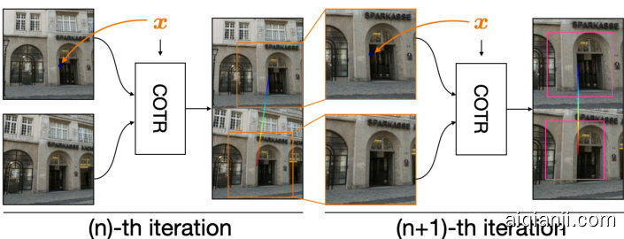
Figure 3. Recursive COTR at inference time – We obtain accurate correspondences by applying our functional approach recursively, zooming into the results of the previous iteration, and running the same network on the pair of zoomed-in crops. We gradually focus on the correct correspondence, with greater accuracy.
图 3: 推理时的递归 COTR —— 我们通过递归应用函数式方法,放大前一次迭代的结果,并在放大后的图像对上运行相同网络,从而获得精确对应关系。随着逐步聚焦于正确对应点,精度也随之提升。
3.3. Inference
3.3. 推理
We next discuss how to apply our functional approach at inference time in order to obtain accurate correspondences.
接下来我们将讨论如何在推理时应用我们的功能方法以获得准确的对应关系。
Inference with recursive with zoom-in. Applying the powerful transformer attention mechanism to vision problems comes at a cost – it requires heavily down sampled feature maps, which in our case naturally translates to poorly localized correspondences; see Section 4.6. We address this by exploiting the functional nature of our approach, applying out network ${\mathcal{F}}_{\Phi}$ recursively. As shown in Fig. 3, we iteratively zoom into a previously estimated correspondence, on both images, in order to obtain a refined estimate. There is a trade-off between compute and the number of zoom-in steps. We ablated this carefully on the validation data and settled on a zoom-in factor of two at each step, with four zoom-in steps. It is worth noting that multiscale refinement is common in many computer vision algorithms [32, 15], but thanks to our functional correspondence model, realizing such a multiscale inference process is not only possible, but also straightforward to implement.
递归放大推理。将强大的Transformer注意力机制应用于视觉问题需要付出代价——它需要大幅下采样的特征图,这在本研究中自然会导致定位对应关系不准确(详见第4.6节)。我们通过利用方法的功能特性,递归应用网络${\mathcal{F}}_{\Phi}$来解决这个问题。如图3所示,我们在两幅图像上对先前估计的对应点进行迭代放大,以获得更精确的估计结果。计算量与放大步骤数之间存在权衡关系,我们在验证数据上进行了细致消融实验,最终确定每步放大两倍,共进行四次放大。值得注意的是,多尺度优化是许多计算机视觉算法的常见策略[32,15],而得益于我们的函数式对应模型,实现这种多尺度推理过程不仅可行,而且实现起来非常直观。
Compensating for scale differences. While matching images recursively, one must account for a potential mismatch in scale between images. We achieve this by making the scale of the patch to crop proportional to the commonly visible regions in each image, which we compute on the first step, using the whole images. To extract this region, we compute the cycle consistency error at the coarsest level, for every pixel, and threshold it at $\tau_{\mathrm{visible}}{=}5$ pixels on the $256\times256$ image; see Fig. 4. In subsequent stages – the zoom-ins – we simply adjust the crop sizes over $\pmb{I}$ and $\pmb{I}^{\prime}$ so that their relationship is proportional to the sum of valid pixels (the unmasked pixels in Fig. 4).
补偿尺度差异。在递归匹配图像时,必须考虑图像间可能存在的尺度不匹配问题。我们通过使裁剪的图块(patch)尺度与每张图像中共同可见区域成比例来实现这一点,该比例关系在第一步使用完整图像计算得出。为提取该区域,我们在最粗粒度层级为每个像素计算循环一致性误差(cycle consistency error),并在$256\times256$图像上以$\tau_{\mathrm{visible}}{=}5$像素为阈值进行二值化处理(见图4)。在后续放大阶段,我们仅需调整$\pmb{I}$和$\pmb{I}^{\prime}$的裁剪尺寸,使其比例关系与有效像素(图4中未掩膜像素)数量总和保持一致。
Dealing with images of arbitrary size. Our network expects images of fixed $256\times256$ shape. To process images of arbitrary size, in the initial step we simply resize (i.e. stretch) them to $256\times256$ , and estimate the initial correspondences. In subsequent zoom-ins, we crop square patches from the original image around the estimated points, of a size commensurate with the current zoom level, and resize them to
处理任意尺寸的图像。我们的网络要求输入固定为 $256\times256$ 尺寸的图像。为处理任意尺寸的图像,初始步骤中我们简单地将其缩放(即拉伸)至 $256\times256$ 并估算初始对应关系。在后续的放大步骤中,我们从原始图像中围绕估算点裁剪出与当前缩放级别相匹配的正方形区域,并将其缩放至

Figure 4. Estimating scale by finding co-visible regions – We show two images we wish to put in correspondence, and the estimated regions in common – image locations with a high cycleconsistency error are masked out.
图 4: 通过寻找共视区域估计尺度——我们展示了两幅需要建立对应关系的图像及其估计的共有区域 (cycle-consistency误差较高的图像区域被掩膜处理)。
$256\times256$ . While this may seem a limitation on images with non-standard aspect ratios, our approach performs well on KITTI, which are extremely wide (3.3:1). Moreover, we present a strategy to tile detections in Section 4.4.
$256\times256$。虽然这看似限制了非标准宽高比的图像,但我们的方法在极宽比例(3.3:1)的KITTI数据集上表现良好。此外,我们将在4.4节提出一种分块检测策略。
Discarding erroneous correspondences. What should we do when we query a point is occluded or outside the viewport in the other image? Similarly to our strategy to compensate for scale, we resolve this problem by simply rejecting correspondences that induce a cycle consistency error (3) greater than $\tau_{\mathrm{cycle}}=5$ pixels. Another heuristic we apply is to terminate correspondences that do not converge while zooming in. We compute the standard deviation of the zoom-in estimates, and reject correspondences that oscillate by more than $\tau_{\mathrm{std}}{=}0.02$ of the long-edge of the image.
丢弃错误对应关系。当查询点在另一图像中被遮挡或位于视口外时,我们该如何处理?与补偿尺度的策略类似,我们通过直接拒绝循环一致性误差 (3) 超过 $\tau_{\mathrm{cycle}}=5$ 像素的对应关系来解决此问题。另一个启发式方法是终止在放大过程中未收敛的对应关系。我们计算放大估计的标准差,并拒绝振荡幅度超过图像长边 $\tau_{\mathrm{std}}{=}0.02$ 的对应关系。
Interpolating for dense correspondence. While we could query every single point in order to obtain dense estimates, it is also possible to densify matches by computing sparse matches first, and then interpolating using bary centric weights on a Delaunay triangulation of the queries. This interpolation can be done efficiently using a GPU rasterizer.
插值实现密集对应。虽然我们可以查询每个点来获取密集估计,但也可以通过先计算稀疏匹配,然后在查询点的Delaunay三角剖分上使用重心权重进行插值来实现匹配的密集化。这种插值可以使用GPU光栅化器高效完成。
3.4. Implementation details
3.4. 实现细节
Datasets. We train our method on the MegaDepth dataset [30], which provides both images and corresponding dense depth maps, generated by SfM [56]. These images come from photo-tourism and show large variations in appearance and viewpoint, which is required to learn invariant models. The accuracy of the depth maps is sufficient to learn accurate local features, as demonstrated by [16, 54, 71]. To find co-visible pairs of images we can train with, we first filter out those with no common 3D points in the SfM model. We then compute the common area between the remaining pairs of images, by projecting pixels from one image to the other. Finally, we compute the intersection over union of the projected pixels, which accounts for different image sizes. We keep, for each image, the 20 image pairs with the largest overlap. This simple procedure results in a good combination of images with a mixture of high/low overlap. We use 115 scenes for training and 1 scene for validation.
数据集。我们在MegaDepth数据集[30]上训练我们的方法,该数据集提供了由SfM[56]生成的图像和相应的密集深度图。这些图像来自照片旅游,展示了外观和视角的巨大变化,这是学习不变模型所必需的。如[16,54,71]所示,深度图的准确性足以学习精确的局部特征。为了找到可以训练的共视图像对,我们首先过滤掉SfM模型中没有共同3D点的图像对。然后,我们通过将像素从一个图像投影到另一个图像来计算剩余图像对之间的共同区域。最后,我们计算投影像素的交并比,以考虑不同的图像大小。对于每个图像,我们保留重叠面积最大的20个图像对。这种简单的程序产生了高/低重叠混合的良好图像组合。我们使用115个场景进行训练,1个场景进行验证。
Implementation. We implement our method in PyTorch [46]. For the backbone $\mathcal{E}$ we use a ResNet50 [23], initialized with weights pre-trained on ImageNet [52]. We use the feature map after its fourth down sampling step (after the third residual block), which is of size $16\times16\times1024.$ , which we convert into $16\times16\times256$ with $1\times1$ convolutions. For the transformer, we use 6 layers for both encoder and decoder. Each encoder layer contains a self-attention layer with 8 heads, and each decoder layer contains an encoder-decoder attention layer with 8 heads, but with no self-attention layers, in order to prevent query points from communicating between each other. Finally, for the network that converts the Transformer output into coordinates, $\mathcal{D}$ , we use a 3-layer MLP, with 256 units each, followed by ReLU activation s.
实现。我们使用PyTorch [46] 实现了我们的方法。对于主干网络 $\mathcal{E}$,我们采用了在ImageNet [52] 上预训练的ResNet50 [23],并取其第四次下采样后的特征图(位于第三个残差块之后),尺寸为 $16\times16\times1024$,随后通过 $1\times1$ 卷积将其转换为 $16\times16\times256$。在Transformer部分,编码器和解码器均使用6层结构。每个编码器层包含一个8头自注意力层,而每个解码器层则包含一个8头编码器-解码器注意力层(不设自注意力层),以避免查询点之间的信息交互。最后,用于将Transformer输出转换为坐标的网络 $\mathcal{D}$ 采用3层MLP(每层256个单元)并接ReLU激活函数。
On-the-fly training data generation. We select training pairs randomly, pick a random query point in the first image, and find its corresponding point on the second image using the ground truth depth maps. We then select a random zoom level among one of ten levels, uniformly spaced, in log scale, between $1\times$ and $10\times$ . We then crop a square patch at the desired zoom level, centered at the query point, from the first image, and a square patch that contains the corresponding point in the second image. Given this pair of crops, we sample 100 random valid correspondences across the two crops – if we cannot gather at least 100 valid points, we discard the pair and move to the next.
动态生成训练数据。我们随机选择训练样本对,在第一张图像中随机选取一个查询点,并使用真实深度图在第二张图像中找到其对应点。随后在$1\times$到$10\times$的对数尺度范围内,从十个均匀分布的缩放级别中随机选择一个级别。接着以查询点为中心,从第一张图像中裁剪出指定缩放倍率的方形图像块,并在第二张图像中裁剪出包含对应点的方形图像块。针对每对图像块,我们在两者之间随机采样100组有效对应点——若无法采集至少100组有效点,则丢弃该样本对并处理下一组数据。
Staged training. Our model is trained in three stages. First, we freeze the pre-trained backbone $\mathcal{E}$ , and train the rest of the network, for $300\mathrm{k\Omega}$ iterations, with the ADAM optimizer [29], a learning rate of $10^{-4}$ , and a batch size of 24. We then unfreeze the backbone and fine-tune everything endto-end with a learning rate of $10^{-5}$ and a batch size of 16, to accommodate the increased memory requirements, for 2M iterations, at which point the validation loss plateaus. Note that in the first two stages we use the whole images, resized to $256\times256$ , as input, which allows us to load the entire dataset into memory. In the third stage we introduce zoom-ins, generated as explained above, and train everything end-to-end for a further $300\mathrm{k}$ iterations.
分阶段训练。我们的模型分三个阶段进行训练。首先,冻结预训练主干网络$\mathcal{E}$,用ADAM优化器[29]、学习率$10^{-4}$、批量大小24训练网络其余部分$300\mathrm{k\Omega}$次迭代。随后解冻主干网络,以学习率$10^{-5}$、批量大小16(为适应更高的内存需求)端到端微调全部网络200万次迭代,直至验证损失趋于平稳。需注意的是,前两个阶段我们使用调整为$256\times256$的完整图像作为输入,这使得我们可以将整个数据集加载到内存中。第三阶段引入上文所述的缩放区域,并端到端训练所有组件额外$300\mathrm{k}$次迭代。
4. Results
- 结果
We evaluate our method with four different datasets, each aimed for a different type of correspondence task. We do not perform any kind of re-training or fine-tuning. They are:
我们用四个不同的数据集评估了我们的方法,每个数据集针对不同类型的对应任务。我们没有进行任何形式的重新训练或微调。这些数据集包括:
• HPatches [2]: A dataset with planar surfaces viewed under different angles/illumination settings, and ground-truth homograph ies. We use this dataset to compare against dense methods that operate on the entire image. • KITTI [19]: A dataset for autonomous driving, where the ground-truth 3D information is collected via LIDAR. With this dataset we compare against dense methods on complex scenes with camera and multi-object motion. • ETH3D [57]: A dataset containing indoor and outdoor scenes captured using a hand-held camera, registered with SfM. As it contains video sequences, we use it to evaluate how methods perform as the baseline widens by increasing the interval between samples, following [69].
• HPatches [2]: 一个包含不同视角/光照条件下平面表面的数据集,并提供真实单应性变换。我们使用该数据集与基于整幅图像的密集方法进行对比。
• KITTI [19]: 用于自动驾驶的数据集,通过激光雷达 (LIDAR) 采集真实3D信息。我们在此数据集上对比相机和多目标运动复杂场景中的密集方法。
• ETH3D [57]: 包含手持相机拍摄的室内外场景数据集,采用运动恢复结构 (SfM) 进行配准。由于包含视频序列,我们参照 [69] 的方法,通过增加采样间隔来评估基线扩大时各算法的性能表现。
| 方法 | AEPE Ex | PCK-1px↑ | PCK-3px↑ | PCK-5px↑ |
|---|---|---|---|---|
| LiteFlowNet[25] CVPR'18 | 118.85 | 13.91 | - | 31.64 |
| PWC-Net[61,62] CVPR'18, TPAMI'19 | 96.14 | 13.14 | - | 37.14 |
| DGC-Net [38] WACV'19 | 33.26 | 12.00 | - | 58.06 |
| GLU-Net[69] CVPR'20 | 25.05 | 39.55 | 71.52 | 78.54 |
| GLU-Net+GOCor[70] NeurIPS'20 | 20.16 | 41.55 | - | 81.43 |
| COTR | 7.75 | 40.91 | 82.37 | 91.10 |
| COTR+Interp. | 7.98 | 33.08 | 77.09 | 86.33 |
Table 1. Quantitative results on HPatches – We report Average End Point Error (AEPE) and Percent of Correct Keypoints (PCK) with different thresholds. For PCK-1px and PCK-5px, we use the numbers reported in literature. We bold the best method and underline the second best.
表 1: HPatches定量评估结果 - 我们报告了不同阈值下的平均端点误差 (AEPE) 和正确关键点百分比 (PCK)。对于PCK-1px和PCK-5px指标,我们采用文献报道的数据。最佳方法用粗体标出,次优方法以下划线标示。
• Image Matching Challenge (IMC2020) [28]: A dataset and challenge containing wide-baseline stereo pairs from photo-tourism images, similar to those we use for training (on MegaDepth). It takes matches as input and measures the quality the poses estimated using said matches. We evaluate our method on the test set and compare against the state of the art in sparse methods.
• Image Matching Challenge (IMC2020) [28]: 一个包含来自照片旅游图像的宽基线立体对数据集及挑战赛,与我们用于训练的数据集 (MegaDepth) 类似。它以匹配点作为输入,并评估基于这些匹配点估计的位姿质量。我们在测试集上评估了该方法,并与稀疏方法领域的先进技术进行了对比。
4.1. HPatches
4.1. HPatches
We follow the evaluation protocol of [69, 70], which computes the Average End Point Error (AEPE) for all valid pixels, and the Percentage of Correct Keypoints (PCK) at a given re projection error threshold – we use 1, 3, and 5 pixels. Image pairs are generated taking the first (out of six) images for each scene as reference, which is matched against the other five. We provide two results for our method: ‘COTR’, which uses 1,000 random query points for each image pair, and ‘COTR $^+$ Interp.’, which interpolates correspondences for the remaining pixels using the strategy presented in Section 3.3. We report our results in Table 1.
我们遵循[69, 70]的评估协议,计算所有有效像素的平均端点误差(AEPE),以及在给定重投影误差阈值下的正确关键点百分比(PCK)——我们使用1、3和5像素作为阈值。图像对生成时,将每个场景的六张图像中的第一张作为参考图像,并与其他五张进行匹配。我们为方法提供了两种结果:"COTR"(每对图像使用1,000个随机查询点)和"COTR$^+$ Interp."(使用第3.3节提出的策略对剩余像素的对应关系进行插值)。结果如 表1 所示。
Our method provides the best results, with and without interpolation, with the exception of PCK-1px, where it remains close to the best baseline. We note that the results for this threshold should be taken with a grain of salt, as several scenes do not satisfy the planar assumption for all pixels. To provide some evidence for this, we reproduce the results for GLU-Net [69] using the code provided by the authors to measure PCK at 3 pixels, which was not computed in the paper. 2 COTR outperforms it by a significant margin.
我们的方法在有无插值情况下均能提供最佳结果,唯独在PCK-1px指标上略逊于最优基线。需要说明的是,该阈值下的结果需谨慎看待,因为部分场景的像素并不完全满足平面假设。为佐证这一点,我们使用作者提供的代码复现了GLU-Net[69]在3像素阈值下的PCK指标(原论文未计算该数据),结果显示COTR以显著优势胜出。
4.2. KITTI
4.2. KITTI
To evaluate our method in an environment more complex than simple planar scenes, we use the KITTI dataset [39, 40]. Following [70, 65], we use the training split for this evaluation, as ground-truth for the test split remains private – all methods, including ours, were trained on a separate dataset. We report results both in terms of AEPE, and ‘Fl.’ – the
为了在比简单平面场景更复杂的环境中评估我们的方法,我们使用了KITTI数据集 [39, 40]。参照 [70, 65] 的做法,本次评估采用训练集划分,因为测试集的真实数据仍未公开——包括本方法在内的所有模型均在独立数据集上完成训练。我们同步汇报了AEPE和"Fl."两项指标结果——

Figure 5. Qualitative examples on KITTI – We show the optical flow and its corresponding error map (“jet” color scheme) for three examples from KITTI-2015, with GLU-Net [69] as a baseline. COTR successfully recovers both the global motion in the scene, and the movement of individual objects, even when nearby cars move in opposite directions (top) or partially occlude each other (bottom).
图 5: KITTI定性示例 – 我们展示了KITTI-2015中三个样本的光流及其对应误差图("jet"配色方案),以GLU-Net [69]作为基线。COTR成功恢复了场景中的全局运动以及单个物体的移动,即使相邻车辆朝相反方向运动(顶部)或部分相互遮挡(底部)。
| 方法 | KITTI-2012 | KITTI-2015 |
|---|---|---|
| AEPE↓ | F1[%]↓ | |
| LiteFlowNet[25] CVPR'18 | 4.00 | 17.47 |
| PWC-Net[61,62] CVPR'18, TPAMI'19 | 4.14 | 20.28 |
| DGC-Net[38] WACV'19 | 8.50 | 32.28 |
| GLU-Net[69] CVPR'20 | 3.34 | 18.93 |
| RAFT[65] ECCV'20 | 2.15 | 9.30 |
| GLU-Net+GOCor[70] NeurIPS'20 | 2.68 | 15.43 |
| COTR3 | 1.28 | 7.36 |
| COTR+Interp. | 2.26 | 10.50 |
Table 2. Quantitative results on KITTI – We report the Average End Point Error (AEPE) and the flow outlier ratio (‘Fl’) on the 2012 and 2015 versions of the KITTI dataset. Our method outperforms most baselines, with the interpolated version being on par with RAFT, and slightly edging out GLU-Net+GOCor.
表 2: KITTI 定量实验结果 - 我们在 KITTI 数据集的 2012 和 2015 版本上报告了平均端点误差 (AEPE) 和光流异常值比率 (Fl) 。我们的方法优于大多数基线,插值版本与 RAFT 相当,并略微优于 GLU-Net+GOCor。
percentage of optical flow outliers. As KITTI images are large, we randomly sample 40,000 points per image pair, from the regions covered by valid ground truth.
光流异常值百分比。由于KITTI图像较大,我们从有效真值覆盖区域中为每对图像随机采样40,000个点。
We report the results on both KITTI-2012 and KITTI2015 in Table 2. Our method outperforms all the baselines by a large margin. Note that the interpolated version also performs similarly to the state of the art, slightly better in terms of flow accuracy, and slightly worse in terms of AEPE, compared to RAFT [65]. It is important to understand here that, while COTR provides a drastic improvement over compared methods, we are evaluating only on points where COTR returns confident results, which is about $81.8%$ of the queried locations – among the $18.2%$ of rejected queries, $67.8%$ fall out of the borders of the other image, which indicates that our filtering is reasonable. This shows that COTR provides highly accurate results in the points we query and retrieve estimates for, and is currently limited by the interpolation strategy. This suggests that improved interpolation strategies based on CNNs, such as those used in [41], would be a promising direction for future research.
我们在表2中报告了KITTI-2012和KITTI2015的测试结果。我们的方法大幅超越了所有基线模型。值得注意的是,插值版本的表现与当前最优方法相当:与RAFT [65]相比,在光流精度上略优,而在AEPE指标上稍逊。需要特别说明的是,虽然COTR相比其他方法取得了显著提升,但我们仅评估了COTR返回高置信度的点位(约占查询点位的81.8%)——在被拒绝的18.2%查询中,有67.8%的点位落在另一幅图像的边界之外,这表明我们的过滤机制是合理的。这说明COTR在我们查询并获取估计值的点位能提供极高精度的结果,当前主要受限于插值策略。这表明基于CNN的改进插值策略(如[41]所采用的方案)将是未来研究的 promising方向。
In Fig. 5 we further highlight cases where our method shows clear advantages over the competitors – we see that the objects in motion, i.e., cars, result in high errors with
在图 5 中,我们进一步展示了本方法相较于竞争对手具有明显优势的案例——可以观察到运动物体(如汽车)会导致较高误差。
Table 3. Quantitative results for ETH3D – We report the Average End Point Error (AEPE) at different sampling “rates” (frame intervals). Our method performs significantly better as the rate increases and the problem becomes more difficult.
| Method | AEPE * | ||||||
| rate=3 | rate=5 | rate=7 | rate=9 | rate=11 | rate=13 | rate=15 | |
| LiteFlowNet[25] CVPR'18 | 1.66 | 2.58 | 6.05 | 12.95 | 29.67 | 52.41 | 74.96 |
| PWC-Net[61,62] CVPR′18, TPAMI 19 | 1.75 | 2.10 | 3.21 | 5.59 | 14.35 | 27.49 | 43.41 |
| DGC-Net[38] WACV°19 | 2.49 | 3.28 | 4.18 | 5.35 | 6.78 | 9.02 | 12.23 |
| GLU-Net[69] CVPR°20 | 1.98 | 2.54 | 3.49 | 4.24 | 5.61 | 7.55 | 10.78 |
| RAFT [65] ECCV'20 | 1.92 | 2.12 | 2.33 | 2.58 | 3.90 | 8.63 | 13.74 |
| COTR | 1.66 | 1.82 | 1.97 | 2.13 | 2.27 | 2.41 | 2.61 |
| COTR+Interp. | 1.71 | 1.92 | 2.16 | 2.47 | 2.85 | 3.23 | 3.76 |
表 3. ETH3D定量结果 - 我们报告了不同采样"率"(帧间隔)下的平均端点误差(AEPE)。随着采样率增加和问题难度提升,我们的方法表现显著优于其他方法。
| 方法 | AEPE * |
|---|---|
| rate=3 | |
| LiteFlowNet[25] CVPR'18 | 1.66 |
| PWC-Net[61,62] CVPR'18, TPAMI 19 | 1.75 |
| DGC-Net[38] WACV'19 | 2.49 |
| GLU-Net[69] CVPR'20 | 1.98 |
| RAFT [65] ECCV'20 | 1.92 |
| COTR | 1.66 |
| COTR+Interp. | 1.71 |
GLU-Net, which is biased towards a single, global motion. Our method, on the other hand, successfully recovers the flow fields for these cases as well, with minor errors at the boundaries, due to interpolation. These examples clearly demonstrate the role that attention plays when estimating correspondences on scenes with moving objects.
GLU-Net偏向于单一的全局运动。相比之下,我们的方法也能成功恢复这些情况下的流场,仅因插值在边界处存在微小误差。这些示例清晰地展现了注意力机制在含运动物体场景中估计对应关系时发挥的作用。
Finally, we stress that while our method is trained on MegaDepth, an urban dataset exhibiting only global, rigid motion, for which ground truth is only available on stationary objects (mostly building facades), our method proves capable of recovering the motion of objects moving in different directions; see Fig. 5, bottom. In other words, it learns to find precise, local correspondences within images, rather than global motion.
最后需要强调的是,虽然我们的方法是在MegaDepth(一个仅呈现全局刚性运动的城市数据集)上训练的,且该数据集的地面真值仅适用于静止物体(主要是建筑立面),但我们的方法被证明能够恢复朝不同方向运动物体的运动状态(见图5底部)。换言之,该方法学会在图像中寻找精确的局部对应关系,而非全局运动。
4.3. ETH3D
4.3. ETH3D
We also report results on the ETH3D dataset, following [69, 70]. This task is closer to the ‘sparse’ scenario, as performance is only evaluated on pixels corresponding to SfM locations with valid ground truth, which are far fewer than for HPatches or KITTI. We summarize the results in terms of AEPE in Table 3, sampling pairs of images with an increasing number of frames between them (the sampling “rate”), which correlates with baseline and, thus, difficulty. Our method produces the most accurate correspondences for every setting, tied with Lite Flow Net [25] at a 3-frame difference, and drastically outperforms every method as the baseline increases4; see qualitative results in Fig. 6.
我们还按照[69, 70]的方法在ETH3D数据集上报告了结果。该任务更接近"稀疏"场景,因为性能评估仅针对具有有效真实值的SfM位置对应的像素点,其数量远少于HPatches或KITTI数据集。我们在表3中以AEPE指标总结了结果,通过逐渐增加采样帧间隔(采样"率")来获取图像对,这与基线长度(即任务难度)相关。我们的方法在所有设置中都生成了最准确的对应关系,其中在3帧间隔时与Lite Flow Net [25]持平,随着基线长度增加4,我们的方法显著优于所有其他方法;定性结果见图6。

Figure 6. Qualitative examples on ETH3D – We show results for GLU-Net [69] and COTR for two examples, one indoors and one outdoors. Correspondences are drawn in green if their re projection error is below 10 pixels, and red otherwise.
图 6: ETH3D定性对比示例 - 我们展示了GLU-Net [69]与COTR在室内外场景的两个案例结果。重投影误差低于10像素的对应点标记为绿色,其余标记为红色。
4.4. Image Matching Challenge
4.4. 图像匹配挑战
Accurate, 6-DOF pose estimation in un constrained urban scenarios remains too challenging a problem for dense methods. We evaluate our method on a popular challenge for pose estimation with local features, which measures performance in terms of the quality of the estimated poses, in terms of mean average accuracy (mAA) at a $5^{\circ}$ and $10^{\circ}$ error threshold; see [28] for details.
在无约束城市场景中实现精确的六自由度 (6-DOF) 姿态估计对于密集方法而言仍极具挑战性。我们在一个基于局部特征的姿态估计挑战赛上评估了所提方法,该挑战通过估计姿态的质量来衡量性能,具体指标为在 $5^{\circ}$ 和 $10^{\circ}$ 误差阈值下的平均精度均值 (mAA) 。详见 [28] 。
We focus on the stereo task.5 As this dataset contains images with un constrained aspect ratios, instead of stretching the image before the first zoom level, we simply resize the short-edge to 256 and tile our coarse, image-level estimates – e.g. an image with 2:1 aspect ratio would invoke two tiling instances. If this process generates overlapping tiles (e.g. with a 4:3 aspect ratio), we choose the estimate that gives best cycle consistency among them. We pair our method with DEGENSAC [12] to retrieve the final pose, as recommended by [28] and done by most participants.
我们专注于立体视觉任务。由于该数据集包含宽高比不受限制的图像,我们不会在第一级缩放前拉伸图像,而是简单地将短边调整为256像素并平铺粗略的图像级估计值(例如,2:1宽高比的图像会触发两个平铺实例)。若此过程产生重叠图块(如4:3宽高比),我们选择其中循环一致性最佳的估计值。根据[28]的建议并遵循多数参赛者做法,我们采用DEGENSAC [12]进行最终位姿检索。
We summarize the results in Table 4. We consider the top performers in the 2020 challenge (a total of 228 entries can be found in the leader boards [link]). As the challenge places a limit on the number of keypoints, instead of matches, we consider both categories (up to 2k and up to $8\mathrm{k\Omega}$ keypoints per image), for fairness – note that our method has no notion of keypoints, instead, we query at random locations.6
我们将结果总结在表4中。我们考虑了2020年挑战赛中表现最佳的方案(排行榜[link]中共有228个参赛作品)。由于该挑战赛对关键点数量而非匹配数量设限,为公平起见,我们同时考虑了两个类别(每张图像最多2k和最多$8\mathrm{k\Omega}$个关键点)——需注意我们的方法没有关键点概念,而是随机位置进行查询。6
With $2\mathrm{k\Omega}$ matches and excluding the methods that feature semantic masking – a heuristic employed in the challenge by
使用 $2\mathrm{k\Omega}$ 匹配并排除那些采用语义掩码 (semantic masking) 的方法——这是在挑战中使用的一种启发式策略。

Figure 7. Qualitative examples for IMC2020 – We visualize the matches produced by COTR (with $N=512$ ) for some stereo pairs in the Image Matching Challenge dataset. Matches are coloured red to green, according to their re projection error (high to low).
图 7: IMC2020定性示例 - 我们可视化展示了COTR (使用$N=512$)在图像匹配挑战数据集中部分立体图像对生成的匹配结果。匹配点根据重投影误差(高到低)由红色渐变至绿色标注。
| 方法 | 内点数↑ | mAA(5°)↑ | mAA(10°)↑ |
|---|---|---|---|
| DoG[34]+HardNet[42]+ModifiedGuidedMatching | 762.0 | 0.476 | - |
| DoG[34]+HardNet[42]+OANet[76]+GuidedMatching | 765.3 | 0.471 | - |
| DoG[34]+HardNet[42]+AdaLAM[11]+DEGENSAC[12] | 627.7 | 0.460 | - |
| DoG[34]+HardNet8[47]+PCA+BatchSampling+DEGENSAC[12] | 583.1 | 0.464 | - |
| SP[13]+SG[54]+DEGENSAC[12]+SemSeg+HAdapt | 441.5 | 0.452 | 0.590 |
| SP[13]+SG[54]+DEGENSAC[12]+SemSeg | 404.7 | 0.429 | 0.568 |
| SP[13]+SG[54]+DEGENSAC[12] | 320.5 | 0.416 | 0.552 |
| DISK[71]+DEGENSAC[12] | 404.2 | 0.388 | 0.513 |
| DoG[34]+HardNet[42]+CustomMatch+DGNSC[12] | 245.4 | 0.369 | 0.492 |
| DoG[34]+HardNet[42]+MAGSAC[3] | 181.8 | 0.318 | 0.438 |
| DoG[34]+LogPolarDesc[17]+DEGENSAC[12] | 162.2 | 0.333 | 0.457 |
| COTR+DEGENSAC12 | 1676.6 | 0.444 | 0.580 |
| COTR+DEGENSAC12 | 840.3 | 0.435 | - |
| COTR+DEGENSAC12 | 421.3 | 0.418 | 0.555 |
| COTR+DEGENSAC12 | 211.7 | 0.392 | 0.529 |
| COTR+DEGENSAC12 | 106.8 | 0.356 | 0.492 |
Table 4. Stereo performance on IMC2020 – We report mean Average Accuracy (mAA) at $5^{\circ}$ and $10^{\circ}$ , and the number of inlier matches, for the top IMC2020 entries, on all test scenes. We highlight the best method in bold and underline the second-best. We exclude entries with components specifically tailored to the challenge, which are enclosed in parentheses, but report them for completeness. Finally, we report results with different number of matches $(N)$ under pure COTR and one entry with 2048 keypoints under COTR guided matching. Pure COTR outperforms all methods in the $2k$ -keypoints category (other than those specifically excluded) with as few as 512 matches per image. With $\otimes$ we indicate clickable URLs to the leader board webpage.
表 4: IMC2020立体匹配性能 - 我们在所有测试场景中报告了IMC2020顶级参赛方案在$5^{\circ}$和$10^{\circ}$下的平均准确率(mAA)及内点匹配数。最佳方法用粗体标出,次优方法加下划线显示。我们排除了专门针对该挑战定制的组件(这些条目用括号标注),但为了完整性仍予以列出。最后,我们报告了纯COTR方法在不同匹配数$(N)$下的结果,以及COTR引导匹配下一个2048关键点的参赛方案。纯COTR在每幅图像仅需512个匹配点时,就在$2k$关键点类别中(除特别排除的方法外)优于所有方法。用$\otimes$标记可点击跳转到排行榜网页的URL。
some participants to filter out keypoints on transient structures such as the sky or pedestrians – COTR ranks second overall. These results showcase the robustness and generality of our method, considering that it was not trained specifically to solve wide-baseline stereo problems. In contrast, the other top entries are engineered towards this specific application. We also provide results lowering the cap on the number of matches (see $N$ in Table 4), showing that our method outperforms vanilla SuperGlue [54] (the winner of the 2k-keypoint category) with as few as 512 input matches, and DISK [71] (the runner-up) with as few as 256 input matches. Qualitative examples on IMC are illustrated in Fig. 7.
一些参与者会过滤掉天空或行人等瞬态结构上的关键点——COTR 在整体排名中位列第二。考虑到我们的方法并非专门针对宽基线立体问题训练,这些结果展示了其鲁棒性和通用性。相比之下,其他排名靠前的方案都是针对这一特定应用进行优化的。我们还提供了减少匹配数量上限的结果(见表 4 中的 $N$),表明我们的方法在仅使用 512 个输入匹配时就优于原始 SuperGlue [54](2k 关键点类别冠军),在仅使用 256 个输入匹配时便超越 DISK [71](亚军)。图 7 展示了 IMC 上的定性示例。
4.5. Object-centric scenes
4.5. 以物体为中心的场景
While our evaluation focuses on outdoor scenes, our models can be applied to very different images, such as those picturing objects. We show one such example in Fig. 8, where COTR successfully estimates dense correspondences for two of objects moving in different directions – despite the fact that this data looks nothing alike the images it was trained with. This shows the generality of our approach.
虽然我们的评估主要针对户外场景,但我们的模型可以应用于截然不同的图像,例如物体照片。我们在图 8 中展示了这样一个示例:尽管数据与训练图像毫无相似之处,COTR 仍成功估计了两个朝不同方向运动物体的密集对应关系。这证明了我们方法的通用性。

Figure 8. Object-centric scenes – We compute dense correspondences with GLU-Net [69] and COTR, and warp the source image to the target image with the resulting flows. GLU-Net fails to capture the bottles being swapped, contrary to our method.
图 8: 以物体为中心的场景 - 我们使用 GLU-Net [69] 和 COTR 计算密集对应关系,并通过生成的流将源图像扭曲到目标图像。与我们的方法不同,GLU-Net 未能捕捉到瓶子被交换的情况。
4.6. Ablation studies
4.6. 消融实验
Filtering. We validate the effectiveness of filtering out bad correspondences (Section 3.3) on the ETH3D dataset, where it improves AEPE by roughly $5%$ relative. More importantly, it effectively removes correspondences with a potentially high error. This allows the dense interpolation step to produce better results. We find that on average $1.2%$ of the correspondences are filtered out on this dataset – below $1%$ up to ‘rate $\scriptstyle=9^{\prime}$ , gradually increasing until $3.65%$ at ‘rate $\mathord{=}15^{\circ}$ On the role of the transformer. Transformers are powerful attention mechanisms, but also costly. It is fair to wonder whether a simpler approach would suffice. We explore the use of MLPs in place of transformers, forming a pipeline similar to [21], and train such a variant – see supplementary material for details. In Fig. 9, we see that the MLP yields globally-smooth estimates, as expected, which fail to model the discontinuities that occur due to 3D geometry. On the other hand, COTR with the transformer successfully aligns source and target even when such discontinuities exist.
过滤。我们在ETH3D数据集上验证了过滤不良对应关系的有效性(第3.3节),相对于基线方法,它将AEPE(平均端点误差)降低了约5%。更重要的是,该方法有效移除了潜在高误差的对应关系,使得密集插值步骤能够产生更好的结果。统计显示,该数据集平均有1.2%的对应关系被过滤——在"rate=9"时低于1%,随着参数增加逐渐上升,至"rate=15"时达到3.65%。
关于Transformer的作用。Transformer是强大的注意力机制,但计算成本较高。我们尝试用MLP替代Transformer构建类似[21]的流程(详见补充材料)。如图9所示,MLP如预期产生全局平滑的估计,但无法建模三维几何导致的间断性。相反,采用Transformer的COTR即使存在几何间断仍能成功对齐源目标。
Zooming. To evaluate how our zooming strategy affects the localization accuracy of the correspondences, we measure the errors in the estimation at each zoom level, in pixels. We use the HPatches dataset, with more granularity than we use for inference, and display the histogram of pixels errors at each zoom level in Fig. 10. As we zoom-in, the distribution shifts to the left and gets squeezed, yielding more accurate estimates. While zooming in more is nearly always beneficial, we found empirically that four zoom-ins with a factor of two at each zoom provides a good balance between compute and accuracy.
放大策略。为评估放大策略对对应关系定位精度的影响,我们以像素为单位测量每个放大级别的估计误差。实验采用比推理阶段更精细的HPatches数据集,图10展示了各放大级别的像素误差直方图。随着放大程度增加,误差分布向左偏移且范围收窄,表明估计精度逐步提升。虽然持续放大几乎总能带来收益,但我们通过实验发现:采用2倍放大系数进行四次放大,能在计算量与精度之间取得最佳平衡。
5. Conclusions and future work
5. 结论与未来工作
We introduced a functional network for image correspondence that is capable to address both sparse and dense matching problems. Through a novel architecture and recursive inference scheme, it achieves performance on par or above the state of the art on HPatches, KITTI, ETH3D, and one scene from IMC2020. As future work, in addition to the improvements we have suggested throughout the paper, we intend to explore the application of COTR to semantic and multimodal matching, and incorporate refinement techniques to further improve the quality of its dense estimates.
我们提出了一种用于图像匹配的功能性网络,能够同时处理稀疏和稠密匹配问题。通过新颖的架构和递归推理方案,该网络在HPatches、KITTI、ETH3D以及IMC2020的一个场景上达到了与当前最优技术相当或更优的性能。作为未来工作方向,除了本文中已提出的改进方案外,我们计划探索COTR在语义匹配和多模态匹配中的应用,并引入优化技术以进一步提升其稠密估计的质量。

Figure 9. Transformer vs MLPs – We show examples of warping the source image onto the target image using estimated dense flows, for two stereo pairs from (top row) the Image Matching Challenge test set and (bottom row) scene $\ '0360'$ of the MegaDepth dataset, which was not used for training nor validation. We use both COTR and a variant replacing the transformer with MLPs. We compute dense correspondences at the coarsest level (for ease of illustration), and use them to warp the source image onto the target image. Note how the MLP cannot capture the various discontinuities that occur due to the non-planar 3D structure, and instead tries to solve the problem with planar warps which produce clear artefacts (top row), and is also unable to match the dome of the palace (bottom row). Our method with the transformer (bottom row) succeeds in both.
图 9: Transformer与MLPs对比——我们展示了使用估计的密集流将源图像扭曲到目标图像的示例,分别来自(顶部)Image Matching Challenge测试集和(底部)MegaDepth数据集中未用于训练或验证的场景$\ '0360'$的立体图像对。我们同时使用了COTR和用MLPs替代transformer的变体。在最粗糙级别计算密集对应(便于说明),并用它们将源图像扭曲到目标图像。请注意,MLP无法捕捉由非平面3D结构引起的各种不连续性,而是试图通过产生明显伪影的平面扭曲来解决问题(顶部),也无法匹配宫殿的圆顶(底部)。而采用transformer的我们的方法(底部)在这两方面都取得了成功。

Figure 10. Zooming – We plot the distribution of the end pixel error (EPE) at different zoom-in levels, on the HPatches dataset. The error clearly decreases as more zoom is applied.
图 10: 放大效果 – 我们在 HPatches 数据集上绘制了不同放大级别下的终点像素误差 (EPE) 分布。随着放大倍数的增加,误差明显减小。
Acknowledgements
致谢
This work was supported by the Natural Sciences and Engineering Research Council of Canada (NSERC) Discovery Grant, Google’s Visual Positioning System, Compute Canada, and Advanced Research Computing at the University of British Columbia.
本研究由加拿大自然科学与工程研究委员会(NSERC)探索基金、谷歌视觉定位系统(Google Visual Positioning System)、加拿大计算平台(Compute Canada)以及不列颠哥伦比亚大学高级研究计算中心(Advanced Research Computing at the University of British Columbia)共同资助。
References
参考文献
COTR: Correspondence Transformer for Matching Across Images
COTR: 跨图像匹配的对应关系Transformer
Supplementary Material
补充材料

Figure B. Unstable training and validation loss for COTR with log-linear positional encoding. We terminate the training earlier as the loss diverges.
图 B: 使用对数线性位置编码的COTR模型训练和验证损失不稳定。由于损失值发散,我们提前终止了训练。

Figure A. Training and validation loss for COTR with linear positional encoding. Both losses slowly converge to a stable status.
图 A: 采用线性位置编码的 COTR 训练与验证损失曲线。两项损失均缓慢收敛至稳定状态。
A. Compute
A. 计算
The functional (and recursive) nature of our approach, coupled with the use of a transformer, means that our method has significant compute requirements. Our currently nonoptimized prototype implementation queries one point at a time, and achieves 35 correspondences per second on a NVIDIA RTX 3090 GPU. This limitation could be addressed by careful engineering in terms of tiling and batching. Our preliminary experiments show no significant drop in performance when we query different points inside a given crop – we could thus potentially process any queries at the coarsest level in a single operation, and drastically reduce the number of operations in the zoom-ins (depending on how many queries overlap in a given crop). We expect this will speed up inference drastically. In addition to batching the queries at inference time, we plan to explore its use on non-random points (such as keypoints) and advanced interpolation techniques.
我们方法的功能性(和递归性)本质,加上使用Transformer,意味着我们的方法对计算资源有较高要求。目前未经优化的原型实现每次查询一个点,在NVIDIA RTX 3090 GPU上每秒可处理35个对应关系。这一限制可以通过精细的工程优化(如分块和批处理)来解决。初步实验表明,在给定裁剪区域内查询不同点时性能没有显著下降——因此我们可能以最粗粒度单次处理所有查询,并大幅减少放大阶段的操作次数(具体取决于给定裁剪区域内查询的重叠情况)。预计这将极大加速推理过程。除了在推理时进行查询批处理外,我们计划探索其在非随机点(如关键点)上的应用以及高级插值技术。
B. Log-linear vs Linear
B. 对数线性与线性
Here, we empirically demonstrate that linear positional encoding is important. We train two COTR models with different positional encoding strategies; see Section 3.2. One model uses log-linear increase in the frequency of the sine/cosine function, and the other uses linear increase instead. Fig. A shows that COTR successfully converges using the linear increase strategy. However, as shown in Fig. B, COTR fails to converge with the commonly used log-linear strategy [73, 10]. We suspect that this is because the task of finding correspondences does not involve very high frequency components, but further investigation is necessary and is left as future work.
我们通过实验证明线性位置编码至关重要。我们训练了两种采用不同位置编码策略的COTR模型(详见第3.2节):一个模型使用正弦/余弦函数的对数线性频率增长策略,另一个则采用线性增长策略。图A显示COTR使用线性增长策略能成功收敛,但如图B所示,采用常用对数线性策略[73,10]时模型无法收敛。我们推测这是因为对应点匹配任务不涉及极高频率成分,但该结论仍需进一步验证,这将作为未来研究方向。
C. Architectural details for COTR
C. COTR 架构细节
Backbone. We use the lower layers of ResNet50 [23] as our CNN backbone. We extract the feature map with 1024 channels after layer3, i.e., after the fourth down sampling step. We then project the feature maps with 1024 channels with $1\times1$ convolution to 256 channels to reduce the amount of computation that happens within the transformers.
主干网络。我们使用ResNet50 [23]的底层作为CNN主干网络。在layer3(即第四次下采样步骤)后提取具有1024个通道的特征图。随后通过$1\times1$卷积将1024通道的特征图投影至256通道,以减少Transformer中的计算量。
Transformers. We use 6 layers in both the transformer encoder and the decoder. Each encoder layer contains an 8- head self-attention module, and each decoder layer contains an 8-head encoder-decoder attention module. Note that we disallow the self-attention in the decoder, in order to maintain the independence between queries – queries should not affect each other.
Transformer。我们在Transformer编码器和解码器中均使用6层结构。每个编码器层包含一个8头自注意力模块,每个解码器层包含一个8头编码器-解码器注意力模块。需要注意的是,我们在解码器中禁用自注意力机制,以保持查询之间的独立性——查询之间不应相互影响。
MLP. Once the transformer decoder process the results, we obtain a 256 dimensional vector that represents where the correspondence should be. We use a 3-layer MLP to regress the corresponding point coordinates from the 256- dimensional latent vector. Each layer contains 256 neurons, followed by ReLU activation s.
MLP。一旦Transformer解码器处理完结果,我们就能得到一个256维向量,表示对应点应该出现的位置。我们使用一个3层MLP从256维潜在向量中回归出对应点的坐标。每层包含256个神经元,后接ReLU激活函数。
D. Architectural details for the MLP variant
D. MLP变体的架构细节
Backbone. We use the same backbone in COTR. The difference here is that, once the feature map with 256 channels is obtained, we apply max pooling to extract the global latent vector for the image, as suggested in [21]. We also tried a variant where we do not apply global pooling and use a fully-connected layer to bring it down to a manageable size of 1024 neurons but it quickly provided degenerate results, where all correspondence estimates were at the centre.
主干网络。我们在 COTR 中使用相同的主干网络。此处的区别在于,一旦获得具有 256 个通道的特征图,我们会按照 [21] 的建议应用最大池化来提取图像的全局潜在向量。我们还尝试了一个变体,即不应用全局池化,而是使用全连接层将其降至可管理的 1024 个神经元大小,但很快出现了退化结果,所有对应估计都集中在中心位置。
MLP. With the latent vectors from each image, we use a 3 layer MLP to regress the correspondence coordinates. Specifically, the input to the coordinate regressor is a 768- dimensional vector, which is the concatenation of two global latent vectors for the input images and the positional encoded query point. Similarly to the MLP used in COTR, each linear layer contains 256 neurons, and followed by ReLU activation s.
MLP。利用每张图像的潜在向量,我们使用一个3层MLP来回归对应坐标。具体而言,坐标回归器的输入是一个768维向量,由输入图像的两个全局潜在向量和位置编码查询点拼接而成。与COTR中使用的MLP类似,每个线性层包含256个神经元,并后接ReLU激活函数。
E. Comparing with RAFT [65]
E. 与 RAFT [65] 的对比
RAFT [65] performs better in KITTI-type of scenarios, not necessarily so for other cases. To show this, we provide results for RAFT [65] on all other datasets in Table A. On KITTI, sparse COTR still performs best, and with the interpolation strategy it is roughly on par with RAFT [65]. On other datasets, COTR outperforms RAFT [65] by a large margin1.
RAFT [65] 在 KITTI 类场景中表现更好,但在其他场景中未必如此。为证明这一点,我们在表 A 中提供了 RAFT [65] 在所有其他数据集上的结果。在 KITTI 上,稀疏 COTR 仍然表现最佳,并且通过插值策略,其性能与 RAFT [65] 大致相当。在其他数据集上,COTR 以显著优势超越 RAFT [65]。
Table A. RAFT on ETH3D, KITTI, HPatches, and IMC2020.
| 方法 | ETH3D | ||||||||
|---|---|---|---|---|---|---|---|---|---|
| AEPE↓ | rate=3 | rate=5 | rate=7 | rate=9 | rate=11 | rate=13 | rate=15 | ||
| RAFT [65] eccv20 | 1.92 | 2.12 | 2.33 | 2.58 | 3.90 | 8.63 | 13.74 | ||
| COTR | 1.66 | 1.82 | 1.97 | 2.13 | 2.27 | 2.41 | 2.61 | ||
| COTR+Interp. | 1.71 | 1.92 | 2.16 | 2.47 | 2.85 | 3.23 | 3.76 |
| 方法 | KITTI 2012 | KITTI 2015 | HPatches | ||||||
|---|---|---|---|---|---|---|---|---|---|
| AEPE↓ | FL↓ | AEPE↓ | AEPE↓ | PCK-1px↑ | PCK-3px↑ | PCK-5px↑ | |||
| RAFT [65] eccv20 | 2.15 | 9.30 | 5.00 | 17.4 | 44.3 | 31.22 | 62.48 | 70.85 | |
| COTR | 1.28 | 7.36 | 2.62 | 9.92 | 7.75 | 40.91 | 82.37 | 91.10 | |
| COTR+Interp. | 2.26 | 10.50 | 6.12 | 16.90 | 7.98 | 33.08 | 77.09 | 86.33 |
| 方法 | Image Matching Challenge | ||||||||
|---|---|---|---|---|---|---|---|---|---|
| Num. Inl.↑ | mAA(5°)↑ | mAA(10°)↑ | |||||||
| RAFT [65] eccv20+DEGENSAC (N=2048) | 1066.1 | 0.163 | |||||||
| COTR+DEGENSAC(N=2048) | 1686.2 |