MCTrack: A Unified 3D Multi-Object Tracking Framework for Autonomous Driving
MCTrack: 自动驾驶的统一3D多目标跟踪框架
Abstract
摘要
This paper introduces MCTrack, a new 3D multi-object tracking method that achieves state-of-the-art (SOTA) performance across KITTI, nuScenes, and Waymo datasets. Addressing the gap in existing tracking paradigms, which often perform well on specific datasets but lack generaliz ability, MCTrack offers a unified solution. Additionally, we have standardized the format of perceptual results across various datasets, termed Base Version, facilitating researchers in the field of multi-object tracking (MOT) to concentrate on the core algorithmic development without the undue burden of data preprocessing. Finally, recognizing the limitations of current evaluation metrics, we propose a novel set that assesses motion information output, such as velocity and acceleration, crucial for downstream tasks. The source codes of the proposed method are available at this link: https://github.com/megvii-research/MCTrack
本文介绍了一种新型3D多目标跟踪方法MCTrack,该方法在KITTI、nuScenes和Waymo数据集上均实现了最先进(SOTA)性能。针对现有跟踪范式在特定数据集表现优异但泛化能力不足的问题,MCTrack提供了统一解决方案。此外,我们统一了各数据集的感知结果格式(称为Base Version),使多目标跟踪(MOT)领域的研究者能专注于核心算法开发,无需承担繁重的数据预处理工作。最后,针对现有评估指标的局限性,我们提出了一套新指标用于评估运动信息输出(如速度和加速度),这对下游任务至关重要。该方法的源代码详见:https://github.com/megvii-research/MCTrack
1. Introduction
1. 引言
3D multi-object tracking plays an essential role in the field of autonomous driving, as it serves as a bridge between perception and planning tasks. The tracking results directly affect the performance of trajectory prediction, which in turn influences the planning and control of the ego vehicle. Currently, common tracking paradigms include tracking-bydetection (TBD) [58, 61, 62], tracking-by-attention (TBA) [14, 48, 69], and joint detection and tracking (JDT) [3, 59]. Generally, the TBD paradigm approach tends to outperform the TBA and JDT paradigm methods in both performance and computational resource efficiency. Commonly used datasets include KITTI [22], Waymo [49], and nuScenes [5], which exhibit significant differences in terms of collection scenarios, regions, weather, and time. Furthermore, the difficulty and format of different datasets vary considerably. Researchers often need to write multiple preprocessing programs to adapt to different datasets. The variability across datasets typically results in these methods attaining SOTA performance solely within the confines of a particular dataset, with less impressive results observed on alternate datasets [26, 31, 32, 54], as shown in Fig.1. For instance, DetZero [36] achieved SOTA performance on the Waymo dataset but was not tested on other datasets. Fast-Poly [32] achieved SOTA performance on the nuScenes dataset but had mediocre performance on the Waymo dataset. Similarly, DeepFusion [58] performed well on the KITTI dataset but exhibited average performance on the nuScenes dataset. Furthermore, in terms of performance evaluation, existing metrics such as CLEAR [4], AMOTA [61], HOTA [35], IDF1 [43], etc., mainly judge whether the trajectory is correctly connected. They fall short, however, in evaluating the precision of subsequent motion information—key information such as velocity, acceleration, and angular velocity—which is crucial for fulfilling the requirements of downstream prediction and planning tasks [31, 54, 58].
3D多目标跟踪在自动驾驶领域发挥着至关重要的作用,它是感知与规划任务之间的桥梁。跟踪结果直接影响轨迹预测的性能,进而影响自车的规划与控制。目前常见的跟踪范式包括检测后跟踪 (TBD) [58, 61, 62]、注意力跟踪 (TBA) [14, 48, 69] 以及联合检测与跟踪 (JDT) [3, 59]。总体而言,TBD范式方法在性能和计算资源效率上往往优于TBA和JDT范式方法。常用数据集包括KITTI [22]、Waymo [49]和nuScenes [5],这些数据集在采集场景、区域、天气和时间方面存在显著差异。此外,不同数据集的难度和格式差异较大,研究人员通常需要编写多个预处理程序以适应不同数据集。数据集的差异性通常导致这些方法仅在特定数据集范围内达到SOTA性能,而在其他数据集上表现平平 [26, 31, 32, 54],如图1所示。例如,DetZero [36]在Waymo数据集上取得了SOTA性能,但未在其他数据集上进行测试;Fast-Poly [32]在nuScenes数据集上表现优异,但在Waymo数据集上表现一般;DeepFusion [58]在KITTI数据集上表现良好,却在nuScenes数据集上呈现平均水平。此外,在性能评估方面,现有指标如CLEAR [4]、AMOTA [61]、HOTA [35]、IDF1 [43]等主要判断轨迹是否正确连接,但未能充分评估后续运动信息(如速度、加速度和角速度等关键信息)的精度,而这些信息对满足下游预测和规划任务的需求至关重要 [31, 54, 58]。
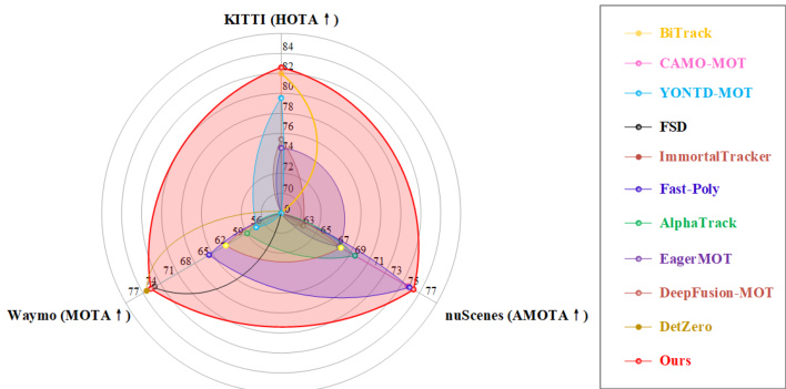
Figure 1. The comparison of the proposed method with SOTA methods across different datasets. For the first time, we have achieved SOTA performance on all three datasets.
图 1: 提出的方法与 SOTA (State Of The Art) 方法在不同数据集上的对比。我们首次在全部三个数据集上实现了 SOTA 性能。
Addressing the noted challenges, we first introduced the Base Version format to standardize perception results (i.e., detections) across different datasets. This unified format greatly aids researchers by allowing them to focus on advancing MOT algorithms, un encumbered by datasetspecific discrepancies.
针对上述挑战,我们首先引入了基础版本 (Base Version) 格式来标准化不同数据集间的感知结果(即检测结果)。这一统一格式使研究人员能专注于推进多目标跟踪 (MOT) 算法发展,无需受限于数据集差异。
Secondly, this paper proposes a unified multi-object tracking framework called MCTrack. To our best knowledge, our method is the first to achieve SOTA performance across the three most popular tracking datasets: KITTI, nuScenes, and Waymo. Specifically, it ranks first in both the KITTI and nuScenes datasets, and second in the Waymo dataset. It is worth noting that the detector used for the firstplace ranking in Waymo dataset is significantly superior to the detector we employed. Moreover, this method is designed from the perspective of practical engineering applications, with the proposed modules addressing real-world issues. For example, our two-stage matching strategy involves the first stage, which performs most of the trajectory matching on the bird’s-eye view (BEV) plane. However, for camera-based perception results, matching on the BEV plane can encounter challenges due to the instability of depth information, which can be as inaccurate as 10 meters in practical engineering scenarios. To address this, trajectories that fail to match in the BEV plane are projected onto the image plane for secondary matching. This process effectively avoids issues such ID-Switch (IDSW) and Fragmentation (Frag) caused by inaccurate depth information, further improving the accuracy and reliability of tracking.
其次,本文提出了一个统一的多目标跟踪框架MCTrack。据我们所知,该方法首次在KITTI、nuScenes和Waymo三大主流跟踪数据集上均达到SOTA性能:具体表现为KITTI和nuScenes双榜第一,Waymo榜单第二。值得注意的是,Waymo榜单第一名使用的检测器性能显著优于我们采用的检测器。该方法的工程设计以实际应用为导向,所提模块均针对现实问题。例如两阶段匹配策略中,第一阶段在鸟瞰图(BEV)平面完成大部分轨迹匹配,但对于基于相机的感知结果,由于深度信息的不稳定性(实际工程中可能存在10米量级的误差),BEV平面匹配可能失效。为此,我们将BEV平面匹配失败的轨迹投影至图像平面进行二次匹配,有效避免了因深度误差导致的ID切换(IDSW)和轨迹断裂(Frag)问题,进一步提升了跟踪的准确性和鲁棒性。
Finally, this paper introduces a set of metrics for evaluating the motion information output by MOT systems, including speed, acceleration, and angular velocity. We hope that researchers will not only focus on the correct linking of trajectories but also consider how to accurately provide the motion information needed for downstream prediction and planning after correct matching, such as speed and acceleration.
最后,本文提出了一套用于评估多目标跟踪(MOT)系统输出运动信息的指标,包括速度、加速度和角速度。我们希望研究者们不仅关注轨迹的正确关联,还能考虑在正确匹配后如何准确提供下游预测和规划所需的运动信息,例如速度和加速度。
2. Related Work
2. 相关工作
2.1. Datasets
2.1. 数据集
Multi-object tracking can be categorized based on spatial dimensions into 2D tracking on the image plane and 3D tracking in the real world. Common datasets for 2D tracking methods include MOT17 [39], MOT20 [15], Dance- Track [50], etc., which typically calculate 2D IoU or appearance feature similarity on the image plane for matching [1, 7, 37]. However, due to the lack of three-dimensional information of objects in the real world, these methods are not suitable for applications like autonomous driving. 3D tracking methods often utilize datasets such as KITTI [22], nuScenes [5], Waymo [49], which provide abundant sensor information to capture the three-dimensional information of objects in the real world. Regrettably, there is a significant format difference among these three datasets, and researchers often need to perform various preprocessing steps to adapt their pipeline, especially for TBD methods, where different detection formats pose a considerable challenge to researchers. To address this issue, this paper standardizes the format of perceptual results (detections) from the three datasets, allowing researchers to focus better on the study of tracking algorithms.
多目标跟踪可根据空间维度分为图像平面上的2D跟踪和现实世界中的3D跟踪。2D跟踪方法常用数据集包括MOT17 [39]、MOT20 [15]、DanceTrack [50]等,这些方法通常通过计算图像平面上的2D IoU或外观特征相似度进行匹配 [1, 7, 37]。然而由于缺乏物体在现实世界中的三维信息,此类方法不适用于自动驾驶等场景。3D跟踪方法常采用KITTI [22]、nuScenes [5]、Waymo [49]等数据集,这些数据集提供丰富的传感器信息以捕捉物体在现实世界中的三维信息。遗憾的是,这三个数据集存在显著的格式差异,研究者往往需要进行各种预处理以适应流程,特别是对于TBD方法而言,不同的检测格式给研究者带来了巨大挑战。为解决该问题,本文统一了三个数据集感知结果(检测)的格式,使研究者能更专注于跟踪算法的研究。
2.2. MOT Paradigm
2.2. MOT范式
Common paradigms in multi-object tracking currently include Tracking-by-Detection (TBD) [58, 70], Joint Detection and Tracking (JDT) [3, 59], Tracking-by-Attention (TBA) [14, 48], and Referring Multi-Object Tracking (RMOT) [19, 63]. JDT, TBA, and RMOT paradigms typically rely on image feature information, requiring GPU resources for processing. However, for the computing power available in current autonomous vehicles, supporting the GPU resources needed for MOT tasks is impractical. Moreover, the performance of these paradigms is often not as effective as the TBD approach. Therefore, this study focuses on TBD-based tracking methods, aiming to design a unified 3D multi-object tracking framework that accommodates the computational constraints of autonomous vehicles.
当前多目标跟踪的常见范式包括检测跟踪(TBD)[58,70]、联合检测跟踪(JDT)[3,59]、注意力跟踪(TBA)[14,48]和指代多目标跟踪(RMOT)[19,63]。JDT、TBA和RMOT范式通常依赖图像特征信息,需要GPU资源进行处理。然而就当前自动驾驶车辆的计算能力而言,支持MOT任务所需的GPU资源并不现实。此外,这些范式的性能往往不如TBD方法。因此,本研究聚焦于基于TBD的跟踪方法,旨在设计一个适应自动驾驶车辆计算限制的统一3D多目标跟踪框架。
2.3. Data Association
2.3. 数据关联
In current 2D and 3D multi-object tracking methods, cost functions such as IoU, GIoU [42], DIoU [72], Euclidean distance, and appearance similarity are commonly used [1, 7]. Some of these cost functions only consider the similarity between two bounding boxes, while others focus solely on the distance between the centers of the boxes. None of them can ensure good performance for each category in every dataset. The Ro GDIoU proposed in this paper, which takes into account both shape similarity and center distance, effectively addresses these issues. Moreover, in terms of matching strategy, most methods adopt a two-stage approach: the first stage uses a set of thresholds for matching, and the second stage relaxes these thresholds for another round of matching. Although this method offers certain improvements, it can still fail when there are significant fluctuations in the perceived depth. Therefore, this paper introduces a secondary matching strategy based on the BEV plane and the Range View (RV) plane, which solves this problem effectively by matching from different perspectives.
在当前2D和3D多目标跟踪方法中,常用IoU、GIoU [42]、DIoU [72]、欧氏距离和外观相似度等成本函数 [1, 7]。其中部分成本函数仅考虑两个边界框之间的相似性,另一些则仅关注框中心距离。这些方法均无法保证在每个数据集的每个类别上都表现良好。本文提出的Ro GDIoU兼顾形状相似性与中心距离,有效解决了上述问题。此外,在匹配策略方面,多数方法采用两阶段方案:第一阶段使用一组阈值进行匹配,第二阶段放宽阈值进行二次匹配。尽管该方法有一定改进,但在感知深度存在显著波动时仍可能失效。为此,本文提出基于BEV平面和Range View (RV)平面的二次匹配策略,通过多视角匹配有效解决了该问题。
2.4. MOT Evaluation Metrics
2.4. MOT 评估指标
The earliest multi-object tracking evaluation metric, CLEAR, was proposed in reference [4], including metrics such as MOTA and MOTP. Subsequently, improvements based on CLEAR have led to the development of IDF1 [43], HOTA [35], AMOTA [61], and so on. These metrics primarily assess the correctness of trajectory connections, that is, whether trajectories are continuous and consistent, and whether there are breaks or ID switches. However, they do not take into account the motion information that must be output after a trajectory is correctly connected in a multiobject tracking task, such as velocity, acceleration, and angular velocity. This motion information is crucial for downstream tasks like trajectory prediction and planning. In light of this, this paper introduces a new set of evaluation metrics that focus on the motion information output by MOT tasks, which we refer to as motion metrics. We encourage researchers in the MOT field to focus not only on the accurate association of trajectories but also on the quality and suitability of the trajectory outputs to meet the requirements of downstream tasks.
最早的多目标跟踪评估指标CLEAR由文献[4]提出,包含MOTA、MOTP等指标。随后基于CLEAR的改进衍生出IDF1 [43]、HOTA [35]、AMOTA [61]等指标。这些指标主要评估轨迹连接的准确性,即轨迹是否连续一致、是否存在断裂或ID切换,但未考虑多目标跟踪任务中轨迹正确连接后必须输出的运动信息(如速度、加速度、角速度)。这些运动信息对轨迹预测、规划等下游任务至关重要。鉴于此,本文提出一套聚焦MOT任务输出运动信息的评估指标,称为运动指标(motion metrics),倡导MOT领域研究者不仅关注轨迹关联的准确性,还应关注轨迹输出的质量与适用性,以满足下游任务需求。
3. MCTrack
3. MCTrack
We present MCTrack, a streamlined, efficient, and unified 3D multi-object tracking method designed for autonomous driving. The overall framework is illustrated in Fig.2, and detailed descriptions of each component are provided below.
我们提出 MCTrack,一种专为自动驾驶设计的简洁、高效且统一的 3D 多目标跟踪方法。整体框架如图 2 所示,各组件的详细描述如下。
3.1. Data Preprocessing
3.1. 数据预处理
To validate the performance of a unified pipeline (PPL) across different datasets and to facilitate its use by researchers, we standardized the format of detection data from various datasets, referring to it as the Base Version format. This format encapsulates the position of obstacles within the global coordinate system, organized by scene ID, frame sequence, and other pertinent parameters. As depicted in Figure 3, the structure includes a comprehensive scene index with all associated frames. Each frame is detailed with frame number, timestamp, unique token, detection boxes, transformation matrix, and additional relevant data.
为验证统一流程(PPL)在不同数据集上的性能并方便研究者使用,我们将各数据集的检测数据格式标准化,称为基础版本格式。该格式通过场景ID、帧序列等参数组织,封装了障碍物在全球坐标系中的位置信息。如图3所示,该结构包含完整的场景索引及关联帧数据。每帧详细记录帧编号、时间戳、唯一Token、检测框、变换矩阵及其他相关数据。
For each detection box, we archive details such as “detection score,” “category,” “global xyz,” “lwh,” “global orientation” (expressed as a quaternion), “global yaw” in radians, “global velocity,” “global acceleration.” For more detailed explanations, please refer to our code repository.
对于每个检测框,我们存档以下详细信息:"检测分数"、"类别"、"全局xyz坐标"、"长宽高(lwh)"、"全局朝向"(以四元数表示)、"全局偏航角"(弧度制)、"全局速度"、"全局加速度"。更详细的说明请参考我们的代码仓库。
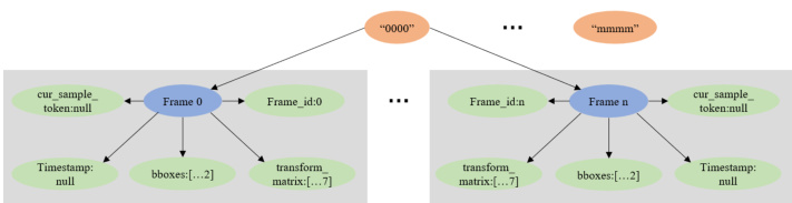
Figure 3. Base Version data format overview.
图 3: 基础版本数据格式概览
3.2. MCTrack Pipeline
3.2. MCTrack 流程
3.2.1 Kalman Filter
3.2.1 卡尔曼滤波器
Currently, most 3D MOT methods [31, 64, 70] incorporate position, size, heading, and score into the Kalman filter modeling, esulting in a state vector $S={x,y,z,l,w,h,\theta,s c o r e,v_{x},v_{y},v_{z}}$ that can have up to 11 dimensions, represented using a unified motion equation, such as constant velocity or constant acceleration models. It is important to note that in this paper, $\theta$ specifically denotes the heading angle. However, this modeling approach has the following issues: Firstly, different state variables may have varying units (e.g., meters, degrees) and magnitudes (e.g., position might be in the meter range, while scores could range from 0 to 1), which can lead to numerical stability problems. Secondly, some state variables exhibit nonlinear relationships (such as the periodic nature of angles), while others are linear (such as dimensions), making it challenging to represent them with a unified motion equation. Furthermore, combining all state variables into a single model increases the dimensionality of the state vector, thereby increasing computational complexity. This may reduce the efficiency of the filter, particularly in real-time applications. Therefore, we decouple the position, size, and heading angle, applying different Kalman filters to each component.
目前,大多数3D MOT方法[31, 64, 70]将位置、尺寸、航向角和得分纳入卡尔曼滤波建模,形成一个最多11维的状态向量 $S={x,y,z,l,w,h,\theta,s c o r e,v_{x},v_{y},v_{z}}$ ,并使用统一运动方程(如匀速或匀加速模型)表示。需注意本文中 $\theta$ 特指航向角。但该建模方式存在以下问题:首先,不同状态变量可能具有不同单位(如米、度)和量级(如位置可能为米级,而得分范围在0到1之间),易导致数值稳定性问题;其次,部分状态变量呈非线性关系(如角度周期性),而另一些是线性的(如尺寸),难以用统一运动方程表征;此外,将所有状态变量合并为单一模型会增加状态向量维度,从而提升计算复杂度,可能降低滤波效率(尤其在实时应用中)。因此,我们将位置、尺寸和航向角解耦,对每个分量应用不同的卡尔曼滤波器。
For position, we only need to model the center point $x,y$ in the BEV plane using a constant acceleration motion model. The state and observation vectors are defined as follows:
对于位置,我们只需在BEV平面上使用恒定加速度运动模型对中心点 $x,y$ 进行建模。状态向量和观测向量定义如下:
$$
S_{\mathsf{p}}={x,y,v_{x},v_{y},a_{x},a_{y}}\quad M_{\mathsf{p}}={x,y,v_{x},v_{y}}
$$
$$
S_{\mathsf{p}}={x,y,v_{x},v_{y},a_{x},a_{y}}\quad M_{\mathsf{p}}={x,y,v_{x},v_{y}}
$$
It should be noted that, theoretically, the size of the same object should remain constant. However, due to potential errors in the perception process, we rely on filters to ensure the stability and continuity of the size.
需要注意的是,理论上同一物体的尺寸应保持恒定。然而,由于感知过程中可能存在误差,我们依赖滤波器来确保尺寸的稳定性和连续性。
Here, $\theta_{p}$ denotes the heading angle provided by perception, while $\theta_{v}$ represents the heading angle calculated from velocity, that is $\theta_{v}=\arctan(v_{y}/v_{x})$ .
这里,$\theta_{p}$ 表示感知提供的航向角,而 $\theta_{v}$ 代表根据速度计算得出的航向角,即 $\theta_{v}=\arctan(v_{y}/v_{x})$。
3.2.2 Cost Function
3.2.2 成本函数
As indicated in reference [73], GIoU fails to distinguish the relative positional relationship when two boxes are con
如文献[73]所述,当两个边界框相...
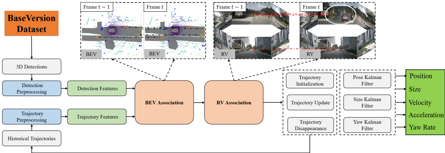
Figure 2. Overview of our unified 3D MOT framework MCTrack. Our input involves converting datasets such as KITTI, nuScenes, and Waymo into a unified format known as Base Version. The entire pipeline operates within the world coordinate system. Initially, we project 3D point coordinates from the world coordinate system onto the BEV plane for the primary matching phase. Subsequently, unmatched trajectory boxes and detection boxes are projected onto the image plane for secondary matching. Finally, the state of the trajectories is updated, along with the Kalman filter. Our output includes motion information such as position, velocity, and acceleration, which are essential for downstream tasks like prediction and planning.
图 2: 我们的统一3D MOT框架MCTrack概述。输入涉及将KITTI、nuScenes和Waymo等数据集转换为统一格式Base Version。整个流程在世界坐标系中运行。首先,我们将世界坐标系中的3D点坐标投影到BEV平面进行主匹配阶段。随后,将未匹配的轨迹框和检测框投影到图像平面进行次匹配。最后更新轨迹状态及卡尔曼滤波器。输出包含位置、速度、加速度等运动信息,这些对预测和规划等下游任务至关重要。
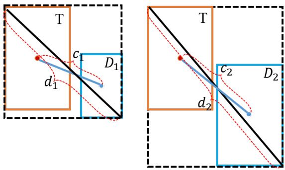
Figure 4. The problem existing in the tracking field with $D I o U$ .
图 4: 跟踪领域存在的 $D I o U$ 问题
When $\frac{c_{1}}{d_{1}}=\frac{c_{2}}{d_{2}}$ is w s tained within one another, effectively reducing to IoU. Similarly, for DIoU, problems also exist, as shown in Fig.4. When the IoU of two boxes is 0 and the center distances are equal, it is also difficult to determine the similarity between the two boxes. Our extensive experiments reveal that using only Euclidean distance or IoU and its variants as the cost metric is inadequate for capturing similarity across all categories. However, combining distance and IoU yields better results. To address these limitations, we propose $R o_G D I o U$ , an IoU variant based on the BEV plane that incorporates the heading angle of the detection box by integrating $G I o U$ and $D I o U$ . Fig.5 shows a schematic of the $R o_G D I o U$ calculation, and the corresponding pseudocode is provided in Algorithm 1.
当 $\frac{c_{1}}{d_{1}}=\frac{c_{2}}{d_{2}}$ 时,两者相互包含,实际上退化为 IoU。类似地,DIoU 也存在问题,如图 4 所示。当两个框的 IoU 为 0 且中心距离相等时,同样难以确定两个框之间的相似性。我们的大量实验表明,仅使用欧氏距离或 IoU 及其变体作为成本度量不足以捕捉所有类别的相似性。然而,结合距离和 IoU 能取得更好的效果。为了解决这些局限性,我们提出了 $R o_G D I o U$,这是一种基于 BEV 平面的 IoU 变体,通过整合 $G I o U$ 和 $D I o U$ 来融入检测框的航向角。图 5 展示了 $R o_G D I o U$ 的计算示意图,相应的伪代码见算法 1。
Where $\omega_{1}$ and $\omega_{2}$ represent the weights for $I o U$ and Euclidean distance respectively, and $\omega_{1}+\omega_{2}=2$ . When two bounding boxes perfectly match, Ro IoU = 1, CC−U = dc22
其中 $\omega_{1}$ 和 $\omega_{2}$ 分别表示 $I o U$ 和欧氏距离的权重,且 $\omega_{1}+\omega_{2}=2$。当两个边界框完全匹配时,Ro IoU = 1,CC−U = dc22
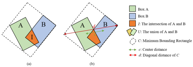
Figure 5. Schematic of Ro GDIoU calculation.
图 5: Ro GDIoU计算示意图。
Algorithm 1: Pseudo-code of Ro GDIoU
算法 1: Ro GDIoU 伪代码
| Input:Detectionboundingbox Bd = (cd,yd,zd,ld, wd,hd,θd) and Trajectory bounding box Bt=(xt,yt,t,lt,wt,ht,θt) Output:Ro_GDIoU Bbev,Bbey = Fglobal→bev(Bd,Bt); Calculate the area ofintersection |
| I = Finter(Bbev, Bbev); Calculate the area of union Calculate the minimum enclosing rectangle C = Frect(Bgev, Bbev); |
| Calculate theEuclideandistancebetween thecenter |
| Calculatethediagonal distance of of theminimum enclosing rectangle d = Fdist (Bbev, Bbev); |
| Ro-IoU = u; Ro-GDIoU = Ro-IoU - w1 · u .3- d2 |
输入:检测边界框 Bd = (cd, yd, zd, ld, wd, hd, θd) 和轨迹边界框 Bt = (xt, yt, t, lt, wt, ht, θt)
输出:Ro_GDIoU
Bbev, Bbey = Fglobal→bev(Bd, Bt);
计算交集面积 I = Finter(Bbev, Bbev);
计算并集面积
计算最小外接矩形 C = Frect(Bgev, Bbev);
计算中心点之间的欧氏距离
计算最小外接矩形的对角线距离 d = Fdist(Bbev, Bbev);
Ro-IoU = u;
Ro-GDIoU = Ro-IoU - w1 · u .3- d2
which means $R o_G D I o U=1$ . When two boxes are far away, $R o_I o U~=~0$ , $\scriptstyle{\frac{C-U}{C}}={\frac{c^{2}}{d^{2}}}\to1$ , which means $R o_G D I o U=-2$ .
这意味着当$R o_G D I o U=1$时。当两个框相距较远时,$R o_I o U~=~0$,$\scriptstyle{\frac{C-U}{C}}={\frac{c^{2}}{d^{2}}}\to1$,即$R o_G D I o U=-2$。
where, $\mathcal{F}(\cdot)$ represents the motion equation, and in this case, we adopt the constant velocity model. The variable $\Delta\tau$ represents the time difference between the current frame and the previous frame.
其中,$\mathcal{F}(\cdot)$ 代表运动方程,此处采用恒定速度模型。变量 $\Delta\tau$ 表示当前帧与前一帧之间的时间差。
The backward prediction can be computed as follows:
反向预测可按如下方式计算:
$$
D_{\tau-1}^{i}=\mathscr{F}^{-1}(x_{\tau}^{\mathrm{d}},y_{\tau}^{\mathrm{d}},v_{{\mathrm{x}},\tau}^{\mathrm{d}},v_{{\mathrm{y}},\tau}^{\mathrm{d}},-\Delta\tau).
$$
$$
D_{\tau-1}^{i}=\mathscr{F}^{-1}(x_{\tau}^{\mathrm{d}},y_{\tau}^{\mathrm{d}},v_{{\mathrm{x}},\tau}^{\mathrm{d}},v_{{\mathrm{y}},\tau}^{\mathrm{d}},-\Delta\tau).
$$
Ultimately, the cost function between the detection box and the trajectory box is computed by the following formula:
最终,检测框与轨迹框之间的成本函数通过以下公式计算:
$$
\mathcal{L}{c o s t}=\alpha\cdot\mathcal{C}(D_{\tau},T_{\tau})+(1-\alpha)\cdot\mathcal{C}(D_{\tau-1},T_{\tau-1}).
$$
$$
\mathcal{L}{c o s t}=\alpha\cdot\mathcal{C}(D_{\tau},T_{\tau})+(1-\alpha)\cdot\mathcal{C}(D_{\tau-1},T_{\tau-1}).
$$
where, $\alpha\in[0,1]$ , and $C$ represents $R o_G D I o U$ .
其中,$\alpha\in[0,1]$,$C$ 表示 $R o_G D I o U$。
3.2.3 Two-Stage Matching
3.2.3 两阶段匹配
Similar to most methods [31, 70], our pipeline also utilizes a two-stage matching process, with the specific flow shown in Pseudocode 2. However, the key difference is that our two-stage matching is performed from different perspectives, rather than by adjusting thresholds within the same perspective.
与大多数方法 [31, 70] 类似,我们的流程同样采用两阶段匹配策略,具体流程如伪代码 2 所示。但关键区别在于:我们的两阶段匹配是从不同视角进行的,而非通过调整同一视角内的阈值实现。
The calculations for $T_{\mathrm{bev}}$ and $D_{\mathrm{{bev}}}$ are illustrated in equation 7. For the calculation of SDIoU, please consult the approach detailed in [57]. We define the coordinate information of the detection or trajectory box as $X=[x,y,z,l,w,h,\theta]$ . According to equation 7, we can determine the corresponding 8 corners, denoted as $C=$ $[P_{0},P_{1},P_{2},P_{3},P_{4},P_{5},P_{6},P_{7}]$ . Among these corners, we select the points with indices [2, 3, 7, 6] to represent the 4 points on the BEV plane.
$T_{\mathrm{bev}}$和$D_{\mathrm{bev}}$的计算如公式7所示。关于SDIoU的计算方法,请参考[57]中详述的方法。我们将检测或轨迹框的坐标信息定义为$X=[x,y,z,l,w,h,\theta]$。根据公式7,可以确定对应的8个角点,记为$C=[P_{0},P_{1},P_{2},P_{3},P_{4},P_{5},P_{6},P_{7}]$。在这些角点中,我们选择索引为[2,3,7,6]的点来表示BEV平面上的4个点。
$$
C=R\cdot P+T.
$$
$$
C=R\cdot P+T.
$$
$$
P=\left[{\frac{l}{2}}{\frac{l}{2}}{\frac{l}{2}}{\frac{l}{2}}{\frac{l}{2}}{\frac{l}{2}}{\frac{l}{3}}{\frac{\ddot{l}}{2}}-{\frac{l}{2}}{\frac{l}{2}}-{\frac{l}{2}}{\frac{\ddot{l}}{2}}-{\frac{l}{2}}{\frac{\ddot{l}}{2}}\right]\nonumber
$$
$$
P=\left[{\frac{l}{2}}{\frac{l}{2}}{\frac{l}{2}}{\frac{l}{2}}{\frac{l}{2}}{\frac{l}{2}}{\frac{l}{3}}{\frac{\ddot{l}}{2}}-{\frac{l}{2}}{\frac{l}{2}}-{\frac{l}{2}}{\frac{\ddot{l}}{2}}-{\frac{l}{2}}{\frac{\ddot{l}}{2}}\right]\nonumber
$$
$$
R=\left[\begin{array}{c c c}{\cos(\theta)}&{-\sin(\theta)}&{0}\ {\sin(\theta)}&{\cos(\theta)}&{0}\ {0}&{0}&{1}\end{array}\right],\quad T=\left[\begin{array}{l}{x}\ {y}\ {z}\end{array}\right].
$$
$$
R=\left[\begin{array}{c c c}{\cos(\theta)}&{-\sin(\theta)}&{0}\ {\sin(\theta)}&{\cos(\theta)}&{0}\ {0}&{0}&{1}\end{array}\right],\quad T=\left[\begin{array}{l}{x}\ {y}\ {z}\end{array}\right].
$$
Algorithm 2: Pseudo-code of Two-stage Matching
算法 2: 两阶段匹配伪代码
| 输入: T-1时刻的轨迹框T, T时刻的检测框D
输出: 匹配索引M
/第一阶段匹配:BEV平面/
Tbev, Dbev = F3d→bev(T, D)
计算代价Lbev = Ro-GDIoU(Dbev, Tbev)
匹配对Mbev = Hungarian(Lbev, thresholdbev)
/第二阶段匹配:RV平面/
for dbev in Dbev do
if dbev not in Mbev[:, 0] then
dbev → Dres
end
end
for tbev in Tbev do
if tbev not in Mbev[:, 1] then
tbev → Tres
end
end
4. New MOT Evaluation Metrics
4. 新型多目标跟踪评估指标
4.1. Static Metrics
4.1. 静态指标
Traditional MOT evaluation primarily relies on metrics such as CLEAR [4], AMOTA [61], HOTA [35], and IDF1 [43]. These metrics focus on assessing the correctness and consistency of trajectory connections. In this paper, we refer to these metrics as static metrics. However, static metrics do not consider the motion information of trajectories after they are connected, such as speed, acceleration, and angular velocity. In fields like autonomous driving and robotics, accurate motion information is crucial for downstream prediction, planning, and control tasks. Therefore, relying solely on static metrics may not fully reflect the actual perfor- mance and application value of a tracking system.
传统多目标跟踪(MOT)评估主要依赖CLEAR [4]、AMOTA [61]、HOTA [35]和IDF1 [43]等指标。这些指标侧重于评估轨迹连接的正确性和一致性。本文将这些指标称为静态指标。然而,静态指标并未考虑轨迹连接后的运动信息,例如速度、加速度和角速度。在自动驾驶和机器人等领域,精确的运动信息对下游预测、规划和控制任务至关重要。因此,仅依赖静态指标可能无法充分反映跟踪系统的实际性能和应用价值。
Introducing motion metrics into MOT evaluation to assess the motion characteristics and accuracy of trajectories becomes particularly important. This not only provides a more comprehensive evaluation of the tracking system’s performance but also enhances its practical application in autonomous driving and robotics, ensuring that the system meets real-world requirements and performs effectively in complex environments.
在MOT评估中引入运动指标以评估轨迹的运动特性和准确性变得尤为重要。这不仅能够更全面地衡量跟踪系统的性能,还能提升其在自动驾驶和机器人领域的实际应用价值,确保系统满足现实需求并在复杂环境中有效运行。
$$
V_{\mathrm{d}}^{S G}=S G\left(V_{\mathrm{d}},w,p\right),
$$
$$
V_{\mathrm{d}}^{S G}=S G\left(V_{\mathrm{d}},w,p\right),
$$
4.2. Motion Metrics
4.2. 运动指标
To address the issue that current MOT evaluation metrics do not adequately consider motion attributes, we propose a series of new motion metrics, including Velocity Angle Error (VAE), Velocity Norm Error (VNE), Velocity Angle Inverse Error (VAIE), Velocity Inversion Ratio (VIR), Velocity Smoothness Error (VSE) and Velocity Delay Error (VDE). These motion metrics aim to comprehensively assess the performance of tracking systems in handling motion features, covering the accuracy and stability of motion information such as speed, angle, and velocity smoothness.
针对当前多目标跟踪(MOT)评估指标未充分考虑运动属性的问题,我们提出了一系列新的运动指标,包括速度角度误差(VAE)、速度范数误差(VNE)、速度角度逆误差(VAIE)、速度反转率(VIR)、速度平滑度误差(VSE)和速度延迟误差(VDE)。这些运动指标旨在全面评估跟踪系统处理运动特征的性能,涵盖速度、角度及速度平滑度等运动信息的准确性和稳定性。
VAE represents the error between the velocity angle obtained from tracking cooperation and the ground truth angle, calculated as:
VAE表示从跟踪合作中获取的速度角度与真实角度之间的误差,计算公式为:
$$
\mathrm{VSE}=|V_{\mathrm{d}}-V_{\mathrm{d}}^{S G})|.
$$
$$
\mathrm{VSE}=|V_{\mathrm{d}}-V_{\mathrm{d}}^{S G})|.
$$
where $w$ and $p$ refer to the window size and polynomial order of the filter, respectively. $V_{\mathrm{d}}^{S G}$ represents the velocity value after being smoothed by the $S G$ filter. A smaller VSE value indicates that the original velocity curve is smoother.
其中 $w$ 和 $p$ 分别表示滤波器的窗口大小和多项式阶数。$V_{\mathrm{d}}^{S G}$ 代表经 $S G$ 滤波器平滑后的速度值。VSE值越小,表明原始速度曲线越平滑。
VDE represents the time delay of the velocity signal obtained by the tracking system relative to the true velocity signal. It is calculated by finding the offset within a given time window, which minimizes the sum of the mean and standard deviation of the difference between the true velocity and the velocity obtained by the tracking system.
VDE表示跟踪系统获取的速度信号相对于真实速度信号的时间延迟。其计算方法是在给定时间窗口内寻找偏移量,使得真实速度与跟踪系统获取速度之差的均值和标准差之和最小。
First, we use a peak detection algorithm to identify the set $v_{g t}^{p}$ of local maxima in the velocity ground truth sequence.
首先,我们使用峰值检测算法来识别速度真实值序列中的局部最大值集合 $v_{g t}^{p}$。
$$
\mathrm{VAE}=(\theta_{g t}-\theta_{d}+\pi)\bmod2\pi-\pi.
$$
$$
\mathrm{VAE}=(\theta_{g t}-\theta_{d}+\pi)\bmod2\pi-\pi.
$$
where $\theta_{\mathrm{gt}}$ denotes the angle calculated from the target speed, and $\theta_{\mathrm{d}}$ denotes the angle calculated from the tracking speed, with both angles ranging from $0^{\circ}$ to $360^{\circ}$ . Given the discontinuity of angles, a $1^{\circ}$ difference from $359^{\circ}$ effectively corresponds to a $2^{\circ}$ separation.
其中 $\theta_{\mathrm{gt}}$ 表示根据目标速度计算的角度,$\theta_{\mathrm{d}}$ 表示根据跟踪速度计算的角度,两个角度的取值范围均为 $0^{\circ}$ 到 $360^{\circ}$。由于角度的不连续性,$359^{\circ}$ 与 $1^{\circ}$ 之间的差值实际上对应 $2^{\circ}$ 的间隔。
VAIE quantifies the angle error when the velocity angle error surpasses a predefined threshold of $\textstyle{\frac{1}{2}}\pi$ . Breaching this threshold typically indicates that the tracking system’s estimation of the target’s velocity direction is directly opposite to the actual direction.
VAIE量化了当速度角度误差超过预设阈值$\textstyle{\frac{1}{2}}\pi$时的角度误差。突破该阈值通常表明跟踪系统对目标速度方向的估计与实际方向完全相反。
$$
\mathrm{VAIE}=\left|\theta_{\mathrm{gt}}-\theta_{\mathrm{d}}\right|,\quad\mathrm{if}\left|\theta_{\mathrm{gt}}-\theta_{\mathrm{d}}\right|>\frac{1}{2}\pi.
$$
$$
\mathrm{VAIE}=\left|\theta_{\mathrm{gt}}-\theta_{\mathrm{d}}\right|,\quad\mathrm{if}\left|\theta_{\mathrm{gt}}-\theta_{\mathrm{d}}\right|>\frac{1}{2}\pi.
$$
The corresponding VIR stands for velocity inverse ratio, which represents the proportion of velocity angle errors that exceed the threshold.
对应的VIR代表速度反比(velocity inverse ratio),表示速度角度误差超过阈值的比例。
where $N$ represents the sequence length of the trajectory.
其中 $N$ 表示轨迹的序列长度。
VNE represents the error between the magnitude of velocity obtained by the tracking system and the true magnitude of velocity, calculated as:
VNE表示跟踪系统获取的速度大小与真实速度大小之间的误差,计算公式为:
$$
\mathrm{VNE}=\left|V_{\mathrm{gt}}-V_{\mathrm{d}}\right|.
$$
$$
\mathrm{VNE}=\left|V_{\mathrm{gt}}-V_{\mathrm{d}}\right|.
$$
where $V_{\mathrm{gt}}$ and $V_{\mathrm{d}}$ represent the actual and predicted velocity magnitudes, respectively.
其中 $V_{\mathrm{gt}}$ 和 $V_{\mathrm{d}}$ 分别表示实际和预测的速度大小。
VSE represents the smoothness error of the velocity obtained from the filter. The smoothed velocity is calculated using the Savitzky-Golay (SG) [45] filter.
VSE 表示从滤波器获得的速度的平滑误差。平滑速度是使用 Savitzky-Golay (SG) [45] 滤波器计算的。
$$
v_{\mathrm{gt}}^{p}={\mathcal{F}}(v_{\mathrm{gt}}),
$$
$$
v_{\mathrm{gt}}^{p}={\mathcal{F}}(v_{\mathrm{gt}}),
$$
Here, ${\mathcal{F}}(\cdot)$ denotes the peak detection function, where the peak points must satisfy the condition $v_{\mathrm{gt}}[t-1]<v_{\mathrm{gt}}[t]>$ $v_{\mathrm{gt}}[t+1]$ . Subsequently, we calculate the difference between the ground truth velocity and the tracking velocity within a given time window.
这里,${\mathcal{F}}(\cdot)$ 表示峰值检测函数,其中峰值点必须满足条件 $v_{\mathrm{gt}}[t-1]<v_{\mathrm{gt}}[t]>$ $v_{\mathrm{gt}}[t+1]$。随后,我们计算给定时间窗口内地面真实速度与跟踪速度之间的差值。
$$
V_{\mathrm{gt}}^{w}=V_{\mathrm{gt}}[t-w/2:t+w/2],
$$
$$
V_{\mathrm{gt}}^{w}=V_{\mathrm{gt}}[t-w/2:t+w/2],
$$
$$
\begin{array}{r}{V_{\mathrm{d},\tau}^{w}=V_{\mathrm{d}}[t-w/2+\tau:t+w/2+\tau],}\ {\tau\in[0,n]\qquad}\end{array}
$$
$$
\begin{array}{r}{V_{\mathrm{d},\tau}^{w}=V_{\mathrm{d}}[t-w/2+\tau:t+w/2+\tau],}\ {\tau\in[0,n]\qquad}\end{array}
$$
$$
\Delta V_{\tau}^{w}={\left\vert v_{\mathrm{gt}}^{i}-v_{\mathrm{d},\tau}^{i}\right\vert\mid(v_{\mathrm{gt}}^{i}\in V_{\mathrm{gt}}^{w},v_{\mathrm{d},\tau}^{i}\in V_{\mathrm{d},\tau}^{w})},
$$
$$
\Delta V_{\tau}^{w}={\left\vert v_{\mathrm{gt}}^{i}-v_{\mathrm{d},\tau}^{i}\right\vert\mid(v_{\mathrm{gt}}^{i}\in V_{\mathrm{gt}}^{w},v_{\mathrm{d},\tau}^{i}\in V_{\mathrm{d},\tau}^{w})},
$$
where $t$ represents the time corresponding to the peak point, $w$ represents the window length, $\tau$ indicates the shift length applied to the velocity window from the tracking system, and $\Delta V_{\tau}^{w}$ represents the set of differences between the true velocity and the tracking velocity. Next, we calculate the mean and standard deviation of set $\Delta V_{\tau}^{w}$ .
其中 $t$ 表示峰值点对应的时间,$w$ 表示窗口长度,$\tau$ 表示跟踪系统中速度窗口应用的偏移长度,$\Delta V_{\tau}^{w}$ 表示真实速度与跟踪速度之间差异的集合。接着,我们计算集合 $\Delta V_{\tau}^{w}$ 的均值和标准差。
$$
M={\mu_{0},\mu_{1},...,\mu_{n}|\mu_{\tau}=\frac{1}{w}\sum_{j=1}^{w}\Delta v_{\tau}^{j}},
$$
$$
M={\mu_{0},\mu_{1},...,\mu_{n}|\mu_{\tau}=\frac{1}{w}\sum_{j=1}^{w}\Delta v_{\tau}^{j}},
$$
$$
\Sigma={\sigma_{0},\sigma_{1},...,\sigma_{n}|\sigma_{\tau}=\sqrt{\frac{1}{w}\sum_{j=1}^{w}\Big(\Delta v_{\tau}^{j}-\mu_{\tau}\Big)^{2}}},
$$
$$
\Sigma={\sigma_{0},\sigma_{1},...,\sigma_{n}|\sigma_{\tau}=\sqrt{\frac{1}{w}\sum_{j=1}^{w}\Big(\Delta v_{\tau}^{j}-\mu_{\tau}\Big)^{2}}},
$$
Finally, the time offset $\tau$ corresponding to the minimum sum of the mean and standard deviation is the VDE.
最后,对应于均值和标准差之和最小的时间偏移 $\tau$ 即为VDE。
$$
\mathrm{VDE}=\tau=\arg\operatorname*{min}_{\tau\in[0,n]}\left(M+\Sigma\right).
$$
$$
\mathrm{VDE}=\tau=\arg\operatorname*{min}_{\tau\in[0,n]}\left(M+\Sigma\right).
$$
where $\tau$ is the timestamp corresponding to the velocity vector and $n$ is the considered time window. It is important to note that for the ground truth of a trajectory, there can be multiple peak points in the time series. The above calculation method only addresses the lag of a single peak point. If there are multiple peak points, the average will be taken to represent the lag of the entire trajectory.
其中 $\tau$ 是对应速度向量的时间戳,$n$ 是考虑的时间窗口。需要注意的是,对于轨迹的真实值,时间序列中可能存在多个峰值点。上述计算方法仅针对单个峰值点的滞后情况。若存在多个峰值点,则将取平均值以代表整条轨迹的滞后量。
To better illustrate the significance of the VDE metric, we provide a schematic diagram in Fig.6. The diagram shows two vehicles traveling at a speed of 100 kilometers per hour: the red one represents the autonomous vehicle, and the white one represents the obstacle ahead. The initial safe distance between the two vehicles is set at 100 meters. Suppose at time point $t_{m}$ , the leading vehicle begins to decelerate urgently and reduces its speed to 60 kilometers per hour by time point $t_{n}$ . If there is a delay in the autonomous vehicle’s perception of the leading vehicle’s speed, it might mistakenly believe that the leading vehicle is still traveling at 100 kilometers per hour. This can lead to an imperceptible reduction in the safe distance between the two vehicles. It is not until time point $t_{n}$ that the autonomous vehicle finally perceives the deceleration of the leading vehicle, by which time the safe distance may be very close to the limit. Therefore, optimizing the motion information output by the multi-object tracking module is also crucial in autonomous driving.
为了更好地说明VDE指标的重要性,我们在图6中提供了示意图。图中展示了两辆以每小时100公里速度行驶的车辆:红色代表自动驾驶车辆,白色代表前方障碍物。两车初始安全距离设定为100米。假设在时间点$t_{m}$,前车开始紧急减速,并在时间点$t_{n}$将速度降至每小时60公里。若自动驾驶车辆对前车速度的感知存在延迟,可能会误判前车仍保持每小时100公里行驶。这将导致两车安全距离出现不易察觉的缩减。直到时间点$t_{n}$,自动驾驶车辆才最终感知到前车减速,此时安全距离可能已接近极限值。因此,优化多目标跟踪模块输出的运动信息对自动驾驶也至关重要。
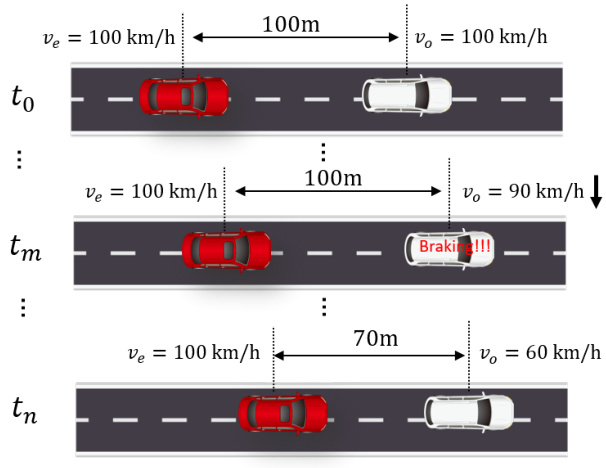
Figure 6. A schematic diagram illustrating the impact of motion information lag on practical applications.
图 6: 运动信息滞后对实际应用影响的示意图。
5. Experiment
5. 实验
In this section, we first outline our experimental setup, including the datasets and implementation details. We then conduct a comprehensive comparison between our method and SOTA approaches on the 3D MOT benchmarks of the KITTI, nuScenes, and Waymo datasets. Following this, we evaluate our newly proposed dynamic metrics using various methods. Finally, we provide a series of ablation studies and related analyses to investigate the various design choices in our approach.
在本节中,我们首先概述实验设置,包括数据集和实现细节。随后在KITTI、nuScenes和Waymo数据集的3D MOT基准测试上,对我们的方法与SOTA方案进行全面比较。接着使用多种方法评估新提出的动态指标。最后通过一系列消融实验和相关分析,探讨方法中的各项设计选择。
5.1. Dataset and Implementation Details
5.1. 数据集与实现细节
A. Datasets
A. 数据集
KITTI: The KITTI tracking benchmark [22] consists of 21 training sequences and 29 testing sequences. The training dataset comprises a total of 8,008 frames, with an average of 3.8 detections per frame, while the testing dataset contains 11,095 frames, with an average of 3.5 detections per frame. The point cloud data in KITTI is captured using a Velodyne HDL-64E LiDAR sensor, with a scan frequency of $10\mathrm{Hz}$ . The time interval $\delta$ between scans, used to infer actual velocity and acceleration, is 0.1 seconds. We compare our results on the vehicle category in the test dataset with those of other methods.
KITTI: KITTI跟踪基准[22]包含21个训练序列和29个测试序列。训练数据集共计8,008帧,平均每帧3.8个检测结果;测试数据集包含11,095帧,平均每帧3.5个检测结果。KITTI中的点云数据由Velodyne HDL-64E激光雷达传感器采集,扫描频率为$10\mathrm{Hz}$。用于推断实际速度和加速度的扫描时间间隔$\delta$为0.1秒。我们在测试数据集的车辆类别上与其他方法进行了结果对比。
NuScenes: The nuScenes dataset [5] is a large-scale dataset that contains 1,000 driving sequences, each spanning 20 seconds. LiDAR data in nuScenes is provided at $20~\mathrm{Hz}$ , but the 3D labels are only available at $2\mathrm{Hz}$ . The nuScenes dataset includes seven categories of data, and we evaluate all of these categories.
NuScenes: nuScenes数据集 [5] 是一个包含1,000段驾驶序列的大规模数据集,每段时长20秒。该数据集中的LiDAR数据以$20~\mathrm{Hz}$频率提供,但3D标注仅以$2\mathrm{Hz}$频率可用。nuScenes数据集涵盖七类数据,我们对所有类别均进行了评估。
Waymo: The Waymo Open Dataset [49] comprises 1,150 sequences, with 798 training sequences, 202 validation sequences, and 150 test sequences. Each sequence con- tains 20 seconds of continuous driving data within a range of $[75\mathrm{m},75\mathrm{m}]$ . The 3D labels are provided for three categories: vehicles, pedestrians, and cyclists. We evaluate all categories in this dataset as well.
Waymo: Waymo开放数据集[49]包含1,150个序列,其中798个训练序列、202个验证序列和150个测试序列。每个序列包含20秒连续驾驶数据,覆盖范围$[75\mathrm{m},75\mathrm{m}]$。该数据集提供三类物体的3D标注:车辆、行人和骑行者。我们同样评估了该数据集的所有类别。
B. Implementation Details
B. 实现细节
Our method is fully implemented in Python on CPU, without the use of GPU acceleration. To ensure optimal performance, during the data preprocessing stage, we filter out bounding boxes with low detection scores and apply Non-Maximum Suppression (NMS) to remove those with significant overlap. We employ three Kalman filters to model the pose, size, and heading angle of the targets, respectively. For the cost calculation, we utilize our newly proposed Ro GDIoU. In our ablation studies, we compare the results obtained using different cost calculation methods. In the matching process, the first match uses the Hungarian algorithm, while the second match employs a greedy algorithm. The ablation study confirms the effectiveness of the double matching approach. In trajectory management, we set different lifecycles for different categories. For more detailed information on hyper parameter settings, please refer to our code implementation.
我们的方法完全基于CPU使用Python语言实现,未采用GPU加速。为确保最佳性能,在数据预处理阶段,我们过滤掉检测分数较低的边界框,并应用非极大值抑制(NMS)消除重叠严重的检测框。我们采用三个卡尔曼滤波器分别对目标姿态、尺寸和航向角进行建模。在成本计算方面,我们使用了新提出的Ro GDIoU方法。消融实验中对比了不同成本计算方法的性能差异。匹配流程采用双重策略:首次匹配使用匈牙利算法,二次匹配采用贪心算法。消融研究证实了双重匹配方案的有效性。轨迹管理模块为不同类别设置了差异化的生命周期周期。具体超参数设置请参阅代码实现。
Table 1. The comparison of the existing methods on the KITTI test set. The best performance is marked in red, and the second-best is marked in blue.
表 1: KITTI测试集上现有方法的对比。最佳性能标红,次佳标蓝。
| 方法 | 检测器 | 模式 | HOTA%↑ | AsSA% | MOTA% | MOTP%↑ | TP↑ | FP↓ | FN↓ | IDS↓ | FRAG↓ |
|---|---|---|---|---|---|---|---|---|---|---|---|
| TripletTrack [38] (CVPR'22) | QD-3DT [25] | online | 73.58 | 74.66 | 84.32 | 86.06 | 29750 | 4642 | 430 | 322 | 522 |
| RAM [51] (ICML'22) | CenterNet [20] | online | 79.53 | 80.94 | 91.61 | 85.79 | 32298 | 2094 | 583 | 210 | 158 |
| FNC2 [29] (TIV'23) | Voxel R-CNN [16] | online | 73.19 | 73.77 | 84.21 | 85.86 | 31629 | 2763 | 2472 | 195 | 301 |
| OC-SORT [7] (CVPR'23) | CenterNet [20] | online | 76.54 | 76.39 | 90.28 | 85.53 | 31707 | 2685 | 407 | 250 | 280 |
| CAMO-MOT [54] (TITS'23) | PointGNN [47] | online | 79.95 | - | 90.38 | 85.00 | - | 2322 | 962 | 23 | - |
| LEGO [71] (arxiv'23) | VirConv [66] | online | 80.75 | 83.27 | 90.61 | 86.66 | 32823 | 1569 | 1445 | 214 | 109 |
| PNAS-MOT [41] (RAL'24) | - | online | 67.32 | 58.99 | 89.59 | 85.44 | 32131 | 2261 | 568 | 751 | 276 |
| SpbTracker [28] (arxiv'24) | DSVT [52] | online | 72.66 | 71.43 | 86.51 | 86.07 | 30884 | 3508 | 875 | 257 | 496 |
| UG3DMOT [24] (SP'24) | CasA [65] | online | 78.60 | 82.28 | 87.98 | 86.56 | 31399 | 2993 | 1111 | 30 | 360 |
| Ours | VirConv [66] | online | 80.78 | 84.30 | 89.82 | 86.71 | 32207 | 2185 | 1252 | 64 | 438 |
| CasTrack [65] (CVPR'22) | CasA [65] | offline | 81.00 | 84.22 | 91.91 | 86.08 | 32859 | 1533 | 1227 | 24 | 107 |
| RethinkMOT [53] (ICRA'23) | PointRCNN [46] | offline | 80.39 | 83.64 | 91.53 | 85.58 | 33094 | 1298 | 1569 | 46 | 134 |
| VirConvTrack [66] (CVPR'23) | VirConv [66] | offline | 81.87 | 86.39 | 90.24 | 86.82 | 31744 | 2648 | 702 | 8 | 77 |
| BiTrack [26] (arxiv'24) | VirConv [66] | offline | 82.39 | 85.57 | 91.52 | 87.55 | 32445 | 1947 | 948 | 20 | 270 |
| Ours | VirConv [66] | offline | 82.56 | 86.64 | 91.62 | 86.82 | 32064 | 2328 | 542 | 12 | 59 |
Table 2. Comparison of existing methods on the nuScenes test set. The best performance is marked in red, and the second-best in blue. Here, (Bic., Motor, Ped., Tra., Tru.) denote (Bicycle, Motorcycle, Pedestrian, Trailer, Truck), and (CR, FC) refer to (Cascade R-CNN [6], FocalsConv [10]).
表 2: nuScenes 测试集上现有方法的对比。最佳性能标红,次佳标蓝。其中 (Bic., Motor, Ped., Tra., Tru.) 表示 (自行车, 摩托车, 行人, 拖车, 卡车), (CR, FC) 指代 (Cascade R-CNN [6], FocalsConv [10])。
| 方法 | 检测器 | AMOTA% | TP↑ | FP↓ | FN↓ | IDS↓ | ||||||||
|---|---|---|---|---|---|---|---|---|---|---|---|---|---|---|
| 总体 | 自行车 | 巴士 | 汽车 | 摩托车 | 行人 | 拖车 | 卡车 | |||||||
| DeepFusionMOT [58] (RAL'22) | CenterPoint[68]&CR[6] | 63.5 | 52.0 | 70.8 | 72.5 | 69.6 | 55.4 | 64.9 | 59.6 | 84304 | 19303 | 33556 | 1075 | |
| SimpleTrack [40] (ECCV'22) | CenterPoint[68] | 66.8 | 40.7 | 71.5 | 82.3 | 67.4 | 79.6 | 67.3 | 58.7 | 95539 | 17514 | 24351 | 575 | |
| MoMA-M3T [27] (CVPR'23) | PGD [56] | 42.5 | 34.1 | 39.5 | 63.4 | 46.4 | 46.9 | 33.0 | 34.6 | 73495 | 18563 | 42934 | 3136 | |
| 3DMOTFormer[17] (ICCV'23) | CenterPoint[68] | 68.2 | 37.4 | 74.9 | 82.1 | 70.5 | 80.7 | 69.6 | 62.6 | 95790 | 18322 | 23337 | 438 | |
| VoxelNeXt[12] (CVPR'23) | VoxelNeXt[12] | 71.0 | 52.6 | 74.7 | 82.6 | 73.1 | 76.0 | 73.8 | 64.4 | 97075 | 18348 | 21836 | 654 | |
| FocalFormal3D-F[13] (ICCV'23) | FocalFormer3D [13] | 73.9 | 54.1 | 79.2 | 83.4 | 74.6 | 84.1 | 75.2 | 66.9 | 97987 | 15547 | 20754 | 824 | |
| MSMDFusion [30] (CVPR'23) | MSMDFusion[30] | 74.0 | 57.4 | 76.7 | 84.9 | 75.4 | 80.7 | 75.4 | 67.1 | 98624 | 14789 | 19853 | 1088 | |
| BEVFusion[34] (ICRA'23) | BEVFusion [34] | 74.1 | 56.0 | 77.9 | 83.1 | 74.8 | 83.7 | 73.4 | 69.5 | 99664 | 19997 | 19395 | 506 | |
| CAMO-MOT[54] (TITS'23) | BEVFusion[34]&FC[10] | 75.3 | 59.2 | 77.7 | 85.8 | 78.2 | 85.8 | 72.3 | 67.7 | 101049 | 17269 | 18192 | 324 | |
| Poly-MOT [31] (ICRA'23) | LargeKernel3D [11] | 75.4 | 58.2 | 78.6 | 86.5 | 81.0 | 82.0 | 75.1 | 66.2 | 101317 | 19673 | 17956 | 292 | |
| CR3DT [2] (arxiv'24) | CR3DT [2] | 35.5 | 23.7 | 30.3 | 56.9 | 42.1 | 33.9 | 27.2 | 34.2 | 62921 | 14428 | 54716 | 1928 | |
| ADA-Track[18] (arxiv'24) | DETR3D[60] | 45.6 | 33.4 | 38.2 | 66.4 | 48.4 | 53.4 | 43.7 | 35.9 | 79051 | 15699 | 39680 | 834 | |
| ShaSTA [44] (RAL'24) | CenterPoint[68] | 69.6 | 41.0 | 73.3 | 83.8 | 72.7 | 81.0 | 70.4 | 65.0 | 97799 | 16746 | 21293 | 473 | |
| NEBP-V3 [33] (TSP'24) | CenterPoint[68]&FC[10] | 74.6 | 49.9 | 78.6 | 86.1 | 80.7 | 83.4 | 76.1 | 67.3 | 99872 | 17243 | 19316 | 377 | |
| Fast-Poly[32] (arxiv'24) | LargeKernel3D [11] | 75.8 | 57.3 | 76.7 | 86.3 | 82.6 | 85.2 | 76.8 | 65.6 | 100824 | 17098 | 18415 | 326 | |
| Ours | LargeKernel3D[11] | 76.3 | 59.1 | 77.2 | 87.9 | 81.9 | 83.2 | 77.9 | 66.7 | 103327 | 19643 | 15996 | 242 |
Table 3. The comparison of the existing algorithms on the Waymo test set. The best performance is marked in red, and the second-best is marked in blue.
表 3: Waymo 测试集上现有算法的对比。最佳性能标红,次佳标蓝。
| Method | Detector | Overall | Vehicle | Pedestrian | Cyclist | MOTP%↓ | FP%↓ | Mismatch% | Miss%↓ |
|---|---|---|---|---|---|---|---|---|---|
| CenterPoint68 | CenterPoint[68] | 58.67 | 59.38 | 56.64 | 60.00 | 25.05 | 9.93 | 0.72 | 30.68 |
| ImmortalTracker55 | CenterPoint[68] | 60.92 | 60.55 | 60.60 | 61.61 | 24.94 | 9.57 | 0.10 | 29.41 |
| SimpleTrack40 | CenterPoint[68] | 60.18 | 60.30 | 60.13 | 60.12 | 24.91 | 9.68 | 0.38 | 29.57 |
| CasTrack65 | CasA[65] | 62.60 | 63.66 | 64.79 | 59.34 | 23.78 | 9.28 | 0.13 | 27.99 |
| YONTD_MOT59 | CenterPoint[68] | 55.70 | 60.48 | 50.08 | 56.55 | 24.07 | 8.44 | 0.60 | 35.26 |
| TrajectoryFormer9 | MPPNet[8] | 66.09 | 65.73 | 66.15 | 66.38 | 23.60 | 10.06 | 0.38 | 23.47 |
| CTRL_FSD_TTA21 | CTRL[21] | 73.29 | 74.29 | 74.21 | 71.37 | 22.80 | 8.45 | 0.04 | 18.21 |
| DetZero36 | DetZero[36] | 75.05 | 75.97 | 76.03 | 73.16 | 22.24 | 7.70 | 0.07 | 17.17 |
| Fast-Poly32 | CasA[65] | 62.77 | 63.06 | 64.92 | 62.77 | 23.74 | 8.71 | 0.12 | 27.59 |
| Ours | CTRL[21] | 73.44 | 74.65 | 74.37 | 71.30 | 22.78 | 8.47 | 0.05 | 18.04 |
5.2. Quantitative Experiment
5.2. 定量实验
We compared MCTrack with published and peer-reviewed SOTA methods on the test sets of the KITTI, nuScenes, and Waymo datasets. Our method demonstrated superior performance across these datasets. Next, we will provide a detailed description of the experimental results on each dataset.
我们在KITTI、nuScenes和Waymo数据集的测试集上将MCTrack与已发表且经过同行评审的SOTA方法进行了比较。我们的方法在这些数据集上均展现出优越性能。接下来将分别详述各数据集的实验结果。
KITTI: On the KITTI dataset, MCTrack demonstrated outstanding performance in both online and offline testing, achieving HOTA scores of $80.78%$ and $82.46%$ respectively, as shown in TABLE 1. These scores are leading among all tested methods. Notably, MCTrack excelled in Association Accuracy (AssA) with a score of $86.55%$ and also displayed the lowest rate of False Negatives (FN). The AssA metric is designed to evaluate the precision of association tasks. Securing the top position in the rankings with our AssA score is a testament to MCTrack’s exceptional ability to accurately match and connect detection targets with high fidelity.
KITTI: 在KITTI数据集上,MCTrack在在线和离线测试中均表现出色,HOTA分数分别达到$80.78%$和$82.46%$,如 表1 所示。这些分数在所有测试方法中处于领先地位。值得注意的是,MCTrack在关联准确率(AssA)方面表现尤为突出,得分为$86.55%$,同时保持了最低的漏检率(FN)。AssA指标专为评估关联任务精度而设计。我们的AssA分数排名第一,充分证明了MCTrack在精确匹配和连接检测目标方面具有卓越的高保真能力。
Furthermore, online tracking performance is particularly crucial in practical engineering applications, as it involves real-time processing and usually does not include subsequent trajectory optimization. In this respect, MCTrack also performed exceptionally well, with its online tracking capabilities being the best among all methods compared.
此外,在线跟踪性能在实际工程应用中尤为关键,因为它涉及实时处理且通常不包含后续轨迹优化。在这方面,MCTrack同样表现卓越,其在线跟踪能力在所有对比方法中最为出色。
NuScenes: On the nuScenes dataset, MCTrack achieved an AMOTA score of $76.3%$ , the best performance among all participating 3D multi-object tracking systems. As shown in TABLE 2. Notably, MCTrack demonstrated superior tracking results in key detection categories such as car and trailer, outperforming other tracking systems. Additionally, for the Kalman filter, we employed only a simple Constant Velocity model. Moreover, MCTrack achieved the highest number of TP and the lowest number of FN and IDS. This result demonstrates MCTrack’s exceptional performance in maintaining tracking stability.
在 nuScenes 数据集上,MCTrack 取得了 $76.3%$ 的 AMOTA 分数,这是所有参赛 3D 多目标跟踪系统中的最佳表现。如 表 2 所示,MCTrack 在关键检测类别(如汽车和拖车)上展现出卓越的跟踪效果,优于其他跟踪系统。此外,对于卡尔曼滤波 (Kalman filter),我们仅采用了简单的恒定速度模型 (Constant Velocity model)。同时,MCTrack 实现了最高的 TP 数量以及最低的 FN 和 IDS 数量。这一结果证明了 MCTrack 在保持跟踪稳定性方面的出色性能。
Waymo: In the Waymo dataset, our method outperforms others when using a unified detector as as show in TABLE 3. Although MCTrack rank second in the leader board, it’s important to note that the detector used by DetZero [36], the top-ranked method, significantly outperforms ours in various metrics, such as a higher mean Average Precision (mAP) by more than two points. We believe that the methods, not only ours but also those of all other ranked methods, are not directly comparable.
Waymo: 在Waymo数据集中,如表3所示,当使用统一检测器时,我们的方法优于其他方法。虽然MCTrack在排行榜上排名第二,但需要注意的是,排名第一的方法DetZero [36]所使用的检测器在多项指标上显著优于我们的检测器,例如平均精度均值(mAP)高出两个点以上。我们认为这些方法(不仅是我们,还包括所有其他上榜方法)并不具备直接可比性。
It is particularly noteworthy that the tracking results we obtained across all three datasets were achieved using the same baseline framework. This fully demonstrates that our baseline framework and methodology not only possess high robustness but also display clear superiority.
特别值得注意的是,我们在所有三个数据集中获得的跟踪结果均使用相同的基线框架实现。这充分证明了我们的基线框架与方法不仅具备高度鲁棒性,还展现出显著优势。
5.3. Motion Metrics Evaluation
5.3. 运动指标评估
In Section 4, we discussed the limitations of existing 3D multi-object tracking metrics and introduced a series of motion metrics. Here, we analyze the results of these motion metrics across different methods. The experiments were conducted on the nuScenes dataset, which includes ground truth speed in its annotations. We used these ground truth values as the reference standard for evaluating our proposed motion metrics. The methods compared include detected speed, speed from differentiation, curve-fitted speed, and Kalman filter-based speed estimation. The comparison results are shown in TABLE 4.
在第4节中,我们讨论了现有3D多目标跟踪指标的局限性,并引入了一系列运动指标。此处,我们分析不同方法在这些运动指标上的结果。实验在nuScenes数据集上进行,该数据集的标注中包含真实速度值。我们以这些真实值作为评估所提运动指标的参考标准。对比方法包括检测速度、微分速度、曲线拟合速度和基于卡尔曼滤波的速度估计。对比结果如 表4 所示。
The velocity obtained through differentiation is calculated based on the change in position and the time difference. The calculation formula is as follows:
通过微分获得的速度是基于位置变化和时间差计算的。计算公式如下:
$$
v_{\mathrm{diff}}=\frac{(x_{\mathrm{cur}}-x_{\mathrm{prev}},y_{\mathrm{cur}}-y_{\mathrm{prev}})}{\Delta t},
$$
$$
v_{\mathrm{diff}}=\frac{(x_{\mathrm{cur}}-x_{\mathrm{prev}},y_{\mathrm{cur}}-y_{\mathrm{prev}})}{\Delta t},
$$
where $(x_{\mathrm{prev}},y_{\mathrm{prev}})$ represents the position of the previous frame, $(x_{\mathrm{cur}},y_{\mathrm{cur}})$ represents the position of the current frame, and $\Delta t$ represents the time difference between the two frames.
其中 $(x_{\mathrm{prev}},y_{\mathrm{prev}})$ 表示前一帧的位置,$(x_{\mathrm{cur}},y_{\mathrm{cur}})$ 表示当前帧的位置,$\Delta t$ 表示两帧之间的时间差。
Curve fitting is based on the positions of the most recent three frames, assuming that the position changes linearly with time. The velocity in each direction is calculated through linear fitting. The linear fitting function is defined as:
曲线拟合基于最近三帧的位置,假设位置随时间线性变化。通过线性拟合计算每个方向的速度。线性拟合函数定义为:
$$
p(x)=a\cdot x+b,
$$
$$
p(x)=a\cdot x+b,
$$
For the $x$ and $y$ coordinates of the position, we perform fitting for frame number $[f_{n-2},f_{n-1},f_{n}]$ and position coordinates $[x_{n-2},x_{n-1},x_{n}]$ and $[y_{n-2},y_{n-1},y_{n}]$ , and the resulting velocity is:
对于位置坐标 $x$ 和 $y$,我们对帧号 $[f_{n-2},f_{n-1},f_{n}]$ 和位置坐标 $[x_{n-2},x_{n-1},x_{n}]$ 及 $[y_{n-2},y_{n-1},y_{n}]$ 进行拟合,所得速度为:
$$
\mathbf{v}{\mathrm{curve}}=\left(a_{x},a_{y}\right).
$$
$$
\mathbf{v}{\mathrm{curve}}=\left(a_{x},a_{y}\right).
$$
The results show that the Kalman filter achieved the lowest VAE and VNE, indicating that it has the highest accuracy in terms of both speed magnitude and direction. Additionally, the Kalman filter also recorded the lowest VIR, demonstrating its ability to effectively suppress speed reversal fluctuations. As expected, the differentiation method resulted in the lowest VDE, indicating the fastest speed response. The curve fitting method, on the other hand, produced the smallest VSE, meaning it generated a smoother speed curve, but at the cost of a larger VSE. As for VAIE, it is difficult to judge its quality solely based on its value, and it typically requires evaluation in the context of practical engineering applications.
结果表明,卡尔曼滤波器实现了最低的VAE和VNE,表明其在速度大小和方向方面具有最高精度。此外,卡尔曼滤波器还记录了最低的VIR,证明其能有效抑制速度反转波动。正如预期,微分法获得了最低的VDE,表明其速度响应最快。而曲线拟合法则产生了最小的VSE,意味着它生成了更平滑的速度曲线,但代价是更大的VSE。至于VAIE,仅凭其值难以判断质量,通常需要结合实际工程应用场景进行评估。
To better explain the meaning of the VDE and VSE metrics, we have created a diagram, as shown in Fig.7. The green curve represents the ground truth velocity, the red curve shows the velocity obtained through differ enc ing, and the blue curve represents the velocity obtained through curve fitting. Compared to curve fitting, the differenced velocity has a faster response, but the smoothness of the curve is inferior. The experimental results also indicate that while the differ enc ing method provides a quicker response, curve fitting generates a much smoother curve.
为了更好地解释VDE和VSE指标的含义,我们绘制了如图7所示的示意图。绿色曲线代表真实速度,红色曲线显示通过差分获得的速度,蓝色曲线表示通过曲线拟合得到的速度。与曲线拟合相比,差分速度具有更快的响应性,但曲线平滑度较差。实验结果也表明,虽然差分方法响应更快,但曲线拟合能生成更为平滑的曲线。
Table 4. The comparison of motion metric results obtained by different methods.
表 4: 不同方法获得的运动指标结果对比
| 方法 | TP↑ | VAE() | VNE(m/s) | VDE(s) | VSE(m/s) | VAIE() | VIR(%)↓ |
|---|---|---|---|---|---|---|---|
| Detection | 88791 | 6.50 | 0.60 | 3.82 | 1.47 | 138.94 | 0.07 |
| Differentiation | 88791 | 8.03 | 0.85 | 3.76 | 1.65 | 137.44 | 0.08 |
| Curve Fitting | 88791 | 8.48 | 2.48 | 4.35 | 0.74 | 137.55 | 0.10 |
| KalmanFilter | 88692 | 6.30 | 0.56 | 3.78 | 1.46 | 141.04 | 0.06 |

Figure 7. Comparison of velocity curves from different methods.
图 7: 不同方法的速度曲线对比。
5.4. Ablation Studies
5.4. 消融实验
To validate the effectiveness of the components in MCTrack, we conducted comprehensive ablation experiments on three datasets: KITTI, nuScenes, and Waymo. For the KITTI dataset, the ablation experiments were performed only on the car category, while for the nuScenes and Waymo datasets, the experiments covered all categories. Our ablation study is divided into two main parts: the first part involves conducting ablation experiments on Ro GDIoU and secondary matching within our unified framework; the second part integrates our Ro GDIoU matching method into other state-of-the-art (SOTA) methods for comparison experiments.
为验证MCTrack中各组件的有效性,我们在KITTI、nuScenes和Waymo三个数据集上进行了全面的消融实验。针对KITTI数据集,消融实验仅针对车辆类别进行;而对nuScenes和Waymo数据集,实验覆盖了所有类别。我们的消融研究分为两个主要部分:第一部分在统一框架内对Ro GDIoU和二次匹配进行消融实验;第二部分将Ro GDIoU匹配方法集成到其他先进(SOTA)方法中进行对比实验。
5.4.1 Pipeline Ablation Studies
5.4.1 流水线消融研究
A. Ro GDIoU
A. Ro GDIoU
We conducted a series of ablation experiments based on the Poly-MOT [31] and PC3T [23] methods on the nuScenes and KITTI datasets, where we replaced the Ro GDIoU in MCTrack with GIoU and DIoU, respectively, to demonstrate the effectiveness and superiority of our cost method. This comparative experiment effectively proves the performance advantages of the proposed method.
我们在 nuScenes 和 KITTI 数据集上基于 Poly-MOT [31] 和 PC3T [23] 方法进行了一系列消融实验,分别用 GIoU 和 DIoU 替换 MCTrack 中的 Ro GDIoU,以验证本文代价度量方法的有效性和优越性。该对比实验有效证明了所提方法的性能优势。
In the experiments on the nuScenes dataset, using Ro GDIoU resulted in improvements of $0.3%$ and $0.9%$ compared to GIoU and DIoU, respectively, fully demonstrating the effectiveness of the Ro GDIoU cost calculation strategy. However, in the experiments on the KITTI dataset, although using Ro GDIoU also improved the HOTA metric compared to GIoU and DIoU, the improvement was not as significant as in the nuScenes dataset. We speculate that this is due to the higher detection accuracy and relatively simpler scenarios in the KITTI dataset, leading to smaller improvements in tracking performance when using Ro GDIoU.
在nuScenes数据集上的实验中,使用Ro GDIoU相比GIoU和DIoU分别带来了$0.3%$和$0.9%$的提升,充分证明了Ro GDIoU成本计算策略的有效性。然而在KITTI数据集的实验中,虽然使用Ro GDIoU相比GIoU和DIoU也提升了HOTA指标,但改进幅度不如nuScenes数据集显著。我们推测这是由于KITTI数据集检测精度更高、场景相对简单,导致使用Ro GDIoU时跟踪性能提升较小。
Table 5. Comparison of results using different cost calculations on MCTrack with the nuScenes dataset (using the Center Point detector [68]).
表 5: 在 nuScenes 数据集上使用不同成本计算方法的 MCTrack 结果对比 (使用 Center Point 检测器 [68])
| 方法 | AMOTA↑ | MOTA↑ | TP↑ | FP↓ | IDS↓ |
|---|---|---|---|---|---|
| MCTrack+GIoU | 73.7 | 63.5 | 84430 | 13851 | 233 |
| MCTrack+DIoU | 73.1 | 62.9 | 85231 | 13332 | 240 |
| MCTrack+Ro_GDIoU | 74.0 | 64.0 | 85900 | 13083 | 275 |
Table 6. Comparison of the best results using different cost calculations on MCTrack with the KITTI training dataset (using the VirConv detector [65]).
表 6: 使用不同成本计算方法在 MCTrack 上与 KITTI 训练数据集的最佳结果对比 (采用 VirConv 检测器 [65])。
| 方法 | HOTA↑ | MOTA↑ | FP↓ | FN↓ | ↑SGI |
|---|---|---|---|---|---|
| MCTrack+ GIoU | 83.55 | 86.17 | 1281 | 2042 | 5 |
| MCTrack + DIoU | 83.69 | 86.37 | 1297 | 1989 | 3 |
| MCTrack+Ro_GDloU | 83.90 | 86.42 | 1261 | 1958 | 3 |
B. Secondary Matching
B. 次级匹配
In practical engineering, obstacles directly in front of a vehicle typically have a much greater impact on driving safety compared to those in other directions. Therefore, to improve efficiency, we project only the obstacles ahead onto the RV plane for secondary matching. Table 7 demonstrates the effectiveness of RV matching on the KITTI dataset. Since these detectors are all based on LiDAR, their depth detection is relatively accurate, and thus RV matching does not lead to significant performance improvements. However, it does improve metrics such as FP and identity IDSW. Interestingly, we observed that the poorer the detector’s performance, the more pronounced the enhancement brought by RV matching, while for the best detectors on the KITTI dataset, the benefits are quite limited. In real-world engineering applications, due to the limited computational resources of autonomous vehicles, their perception performance often falls short of what is demonstrated in opensource datasets. Therefore, we believe that RV matching technology can enhance perception performance in practical scenarios.
在实际工程中,车辆正前方的障碍物通常比其他方向的障碍物对行车安全的影响更大。因此,为提高效率,我们仅将前方障碍物投影到RV平面进行二次匹配。表7展示了在KITTI数据集上RV匹配的效果。由于这些检测器均基于LiDAR,其深度检测相对准确,因此RV匹配并未带来显著的性能提升,但对FP和身份IDSW等指标有所改善。有趣的是,我们发现检测器性能越差,RV匹配带来的提升越明显,而对于KITTI数据集上表现最优的检测器,其增益则相当有限。在现实工程应用中,由于自动驾驶车辆计算资源有限,其感知性能往往达不到开源数据集展示的水平。因此,我们认为RV匹配技术能够提升实际场景中的感知性能。
Table 7. Ablation experiments of secondary matching based on RV across different detectors, where BEV refers to matching on the BEV plane and RV refers to matching on the RV plane.
表 7. 基于RV平面的二次匹配消融实验对比结果,其中BEV表示在BEV平面上进行匹配,RV表示在RV平面上进行匹配。
| 检测器 | BEV | RV | MOTA↑ | FN↓ | FP↓ | IDS↓ |
|---|---|---|---|---|---|---|
| PR [46] | x | 63.5 | 2467 | 6240 | 65 | |
| PR [46] | √ | √ | 64.2 | 2488 | 6087 | 60 |
| SECOND [67] | √ | x | 79.3 | 4216 | 715 | 50 |
| SECOND [67] | √ | 79.5 | 4219 | 695 | 45 | |
| CasA [65] | √ | x | 83.9 | 1933 | 1902 | 30 |
| CasA [65] | √ | √ | 84.1 | 1937 | 1874 | 29 |
| VirConv [66] | √ | 85.9 | 2097 | 1279 | 24 | |
| VirConv [66] | 85.9 | 2097 | 1276 | 24 |
5.4.2 Ro GDIoU for other methods
5.4.2 其他方法的 Ro GDIoU
To further validate the effectiveness of the proposed Ro GDIoU, we integrated it into two SOTA tracking methods, Poly-MOT and PC3T, which are widely used in the nuScenes and KITTI open-source communities. By incorporating Ro GDIoU into these established frameworks, we aimed to assess its impact on improving tracking accuracy and robustness across different datasets and real-world scenarios. The integration allows for a more comprehensive evaluation of Ro GDIoU’s performance, demonstrating its potential to enhance the precision of object tracking in challenging environments. The results of these experiments are presented in TABLE 8 and TABLE 9.
为进一步验证所提出的Ro GDIoU有效性,我们将其集成至nuScenes和KITTI开源社区广泛使用的两种SOTA跟踪方法Poly-MOT与PC3T中。通过将Ro GDIoU融入这些成熟框架,我们旨在评估其在不同数据集和现实场景中对跟踪精度与鲁棒性的提升效果。该集成方案能更全面地评估Ro GDIoU性能,证明其在复杂环境下提升目标跟踪精度的潜力。实验结果展示于表8和表9。
Table 8. Comparison of results on the nuScenes dataset after replacing Poly-MOT’s cost calculation with Ro GDIoU.
表 8: 在 nuScenes 数据集上用 Ro GDIoU 替换 Poly-MOT 成本计算后的结果对比
| 方法 | 使用 Ro | AMOTA%↑ | MOTA%↑ | TP↑ | FP↓ | IDS↓ |
|---|---|---|---|---|---|---|
| PolyMOT [31] | 73.1 | 61.9 | 84072 | 13051 | 232 | |
| PolyMOT [31] | √ | 73.5 | 63.0 | 84624 | 13164 | 279 |
Table 9. Comparison of results on the KITTI training dataset after replacing PC3T’s cost calculation with Ro GDIoU.
表 9: 在KITTI训练数据集上用Ro GDIoU替换PC3T成本计算后的结果对比
| 方法 | w/Ro | HOTA%↑ | MOTA%↑ | ↑NI | ↑SII | |
|---|---|---|---|---|---|---|
| PC3T [64] | 83.17 | 86.07 | 1348 | 1992 | 13 | |
| PC3T [64] | 83.65 | 86.32 | 1252 | 2038 | 3 | |
| DFMOT [58] | 77.45 | 87.27 | 643 | 2337 | 76 | |
| DFMOT [58] | √ | 77.76 | 87.29 | 724 | 2282 | 54 |
The results clearly demonstrate that Ro GDIoU brings a substantial improvement to the performance of the original tracking algorithms on both the KITTI and nuScenes datasets. By integrating Ro GDIoU, the algorithms achieve higher accuracy in object detection and association, leading to more reliable and precise tracking, especially in complex scenarios.
结果清楚地表明,Ro GDIoU 显著提升了原始跟踪算法在 KITTI 和 nuScenes 数据集上的性能。通过集成 Ro GDIoU,算法在目标检测与关联中实现了更高精度,尤其在复杂场景下能提供更可靠、更精准的跟踪效果。
6. Conclusion
6. 结论
In this work, we have developed a concise and unified 3D multi-object tracking method specifically tailored for the autonomous driving domain. Our approach has achieved SOTA performance across various datasets. Furthermore, we have standardized the perception formats of different datasets, allowing researchers to focus on the study of multi-object tracking algorithms without dealing with the cumbersome preprocessing work caused by format differences between datasets. Lastly, we have introduced a new set of evaluation metrics aimed at measuring the performance of multi-object tracking, encouraging researchers to pay attention not only to the correct matching of trajectories but also to the performance of motion attributes essential for downstream applications.
在这项工作中,我们开发了一种简洁统一的3D多目标跟踪方法,专门针对自动驾驶领域。我们的方法在多个数据集上实现了SOTA(当前最优)性能。此外,我们标准化了不同数据集的感知格式,使研究人员能够专注于多目标跟踪算法的研究,而无需处理数据集间格式差异带来的繁琐预处理工作。最后,我们引入了一套新的评估指标,旨在衡量多目标跟踪的性能,鼓励研究人员不仅关注轨迹的正确匹配,还要关注对下游应用至关重要的运动属性表现。